Model and source
- Citation: Hirt D, Urien S, Olivier M, Peyriere H, Nacro B, Diagbouga S, Zoure E, Rouet F, Hien H, Msellati P, Van De Perre P, Treluyer JM. Is the recommended dose of efavirenz optimal in young West African human immunodeficiency virus-infected children? Antimicrob Agents Chemother. 2009;53(10):4407-4413. doi:10.1128/AAC.01594-08
- Description: One-compartment population PK model with first-order absorption and elimination for once-daily oral efavirenz (EFV) in treatment-naive HIV-1-infected West African children (Hirt 2009). CL/F and V/F scale linearly with body weight (shared allometric exponent fixed at 1) and CL/F additionally varies with postnatal age via a power covariate centred at the cohort median 6.35 years (signed exponent -0.535, so apparent clearance decreases with age); the inter-individual variability of V/F is forced to perfect correlation with the eta of CL/F and is constructed as vc_eta_scale * etalcl (the K parameter in Hirt 2009 Table 2); multiplicative residual error.
- Article: https://doi.org/10.1128/AAC.01594-08
Population
The model was developed from 200 plasma efavirenz concentrations
collected in 48 treatment-naive HIV-1-infected West African children
enrolled in the BURKINAME-ANRS 12103 phase II open-label trial
(NCT00122538) in Bobo-Dioulasso, Burkina Faso. Cohort median age was
6.35 years (range 2.77-14.70), median body weight 16.4 kg (range 11-37),
and median height 106 cm (range 85-150); all subjects were Black African
and the original analysis could not test ethnicity as a covariate.
Children received once-daily oral efavirenz as 200 mg capsules, dosed by
body-weight band per the pediatric label, alongside once-daily
didanosine (240 mg/m^2 BSA) and lamivudine (8 mg/kg). Sampling at week 2
was sparse (pre-dose, 1 h, 3 h post-dose) and a richer 24 h profile
(pre-dose, 1, 2, 3, 6, 12, 24 h) was collected between months 2 and 5
for 9 of the 48 children. EFV plasma concentrations were measured by
HPLC-UV (LLOQ 0.5 mg/L); no observation fell below LLOQ. See Hirt 2009
Table 1 for the cohort baseline characteristics and Methods ‘Patients’
for the eligibility criteria. The same information is available
programmatically via
readModelDb("Hirt_2009_efavirenz")$population.
Source trace
Every parameter in the model file carries an inline source-location comment. The table below collects the entries in one place for review.
| Equation / parameter | Value | Source location |
|---|---|---|
lka (ka) |
0.45 1/h | Table 2, Final model, ka row (RSE 23%) |
lcl (CL/F per kg, multiplied by reference WT 16.4
kg) |
0.21 L/h/kg | Table 2, Final model, CL/F row (RSE 9%) |
lvc (V/F per kg, multiplied by reference WT 16.4
kg) |
4.48 L/kg | Table 2, Final model, V/F row (RSE 14%) |
e_wt_cl_vc (shared linear WT exponent on CL/F and V/F;
fixed) |
1 | Discussion paragraph 3 on page 4410 |
e_age_cl (age power exponent on CL/F) |
-0.535 | Table 2, Final model, theta_age = 0.54 (RSE 28%); page 4410 reports 0.535 with the age term in the denominator |
vc_eta_scale (K coupling for eta_V/F = K *
eta_CL/F) |
0.64 | Table 2, Final model, K row (RSE 10%) |
| IIV CL/F (omega^2 = log(1 + 0.61^2) = 0.31634) | 61% CV | Table 2, Final model, omega(CL/F) row (RSE 19%) |
| Proportional residual error sigma | 35% | Table 2, Final model, sigma row (RSE 13%) |
| CL/F covariate equation | – | Results paragraph ‘Population pharmacokinetics’ and equations on p. 4410 (CL/F = theta_CL/F * BW / (age/6.35)^0.535) |
| V/F covariate equation | – | Results paragraph ‘Population pharmacokinetics’ and equations on p. 4410 (V/F = theta_V/F * BW) |
| Perfect-correlation IIV reparameterisation | – | Results paragraph ‘Population pharmacokinetics’ on p. 4410 (‘CL/F = theta_CL/F * exp(eta_CL/F) and V/F = theta_V/F * exp(eta_CL/F * K)’) |
| 1-cmt structure, oral first-order absorption | – | Results paragraph ‘Population pharmacokinetics’; NONMEM ADVAN2 TRANS2 |
Virtual cohort
The published patient-level data are not openly available; the virtual cohorts below mirror the BURKINAME-ANRS 12103 demographics in Hirt 2009 Table 1. Two cohorts are used.
- Whole-cohort VPC – 400 children sampled from a continuous covariate distribution that spans the trial’s age and weight ranges. Used to replicate the visual predictive check standardised to a 250 mg dose (Hirt 2009 Figure 3) and to drive the PKNCA validation against Table 3.
- Age x dose grid (Figure 4 reproduction) – 6 age strata (2-4, 4-6, 6-8, 8-10, 10-12, 12-15 years) x 4 once-daily mg/kg doses (10, 15, 20, 25 mg/kg) x 150 children per stratum. Within each age stratum, body weight is sampled from a WHO weight-for-age-band lognormal centred at the midpoint of the WHO reference weight band, so the virtual children have biologically plausible (age, weight) pairs rather than an unconditional joint sample.
set.seed(20091015)

# Whole-cohort VPC: 400 children spanning the trial's joint (age, weight)
# distribution. AGE log-normal centred at the cohort median 6.35 y; WT
# correlated with AGE via a simple linear regression (the trial reported
# median weight 16.4 kg at median age 6.35 y; slope of ~1.7 kg/y is a
# rough fit to pediatric weight-for-age curves over 2-15 y).
n_vpc <- 400L
age_vpc <- pmin(pmax(exp(rnorm(n_vpc, log(6.35), 0.45)), 2.77), 14.70)
wt_vpc  <- pmin(pmax(16.4 + 1.7 * (age_vpc - 6.35) +
                       rnorm(n_vpc, 0, 2.5), 11), 37)

demo_vpc <- tibble(
  id   = seq_len(n_vpc),
  WT   = wt_vpc,
  AGE  = age_vpc,
  dose_mg = 250,         # Hirt 2009 Figure 3 standardises to a 250 mg dose
  cohort  = "VPC 250 mg"
)

# Figure 4 grid: 6 age strata x 4 mg/kg doses. WHO weight-for-age band
# midpoints (kg) for the centre of each age stratum:
#   3 y  -> 14 kg, 5 y  -> 18 kg, 7 y  -> 23 kg
#   9 y  -> 28 kg, 11 y -> 35 kg, 13 y -> 45 kg
# (Approximate; the BURKINAME cohort was on the lighter end of these bands.)
age_strata <- tibble::tribble(
  ~age_label,  ~age_low, ~age_high, ~age_mid, ~wt_mid,
  "2-4 y",      2,        4,        3,        14,
  "4-6 y",      4,        6,        5,        18,
  "6-8 y",      6,        8,        7,        23,
  "8-10 y",     8,        10,       9,        28,
  "10-12 y",    10,       12,       11,       35,
  "12-15 y",    12,       15,       13,       45
)
dose_levels <- c(10, 15, 20, 25)  # mg/kg once daily

n_per_stratum <- 150L

make_fig4_cohort <- function(age_label, age_low, age_high, age_mid, wt_mid,
                              dose_mg_per_kg, id_offset) {
  ages    <- pmin(pmax(rnorm(n_per_stratum, age_mid, (age_high - age_low) / 4),
                       age_low), age_high)
  weights <- pmin(pmax(exp(rnorm(n_per_stratum, log(wt_mid), 0.12)),
                       0.6 * wt_mid), 1.6 * wt_mid)
  tibble(
    id       = id_offset + seq_len(n_per_stratum),
    WT       = weights,
    AGE      = ages,
    dose_mg  = round(dose_mg_per_kg * weights, 1),
    mg_kg    = dose_mg_per_kg,
    age_label = factor(age_label,
                       levels = c("2-4 y", "4-6 y", "6-8 y",
                                  "8-10 y", "10-12 y", "12-15 y")),
    cohort   = sprintf("%s @ %d mg/kg", age_label, dose_mg_per_kg)
  )
}

grid_fig4 <- tidyr::crossing(age_strata, dose_mg_per_kg = dose_levels) |>
  arrange(age_label, dose_mg_per_kg) |>
  mutate(id_offset = (row_number() - 1L) * n_per_stratum)

demo_fig4 <- purrr::pmap_dfr(
  list(age_label      = grid_fig4$age_label,
       age_low        = grid_fig4$age_low,
       age_high       = grid_fig4$age_high,
       age_mid        = grid_fig4$age_mid,
       wt_mid         = grid_fig4$wt_mid,
       dose_mg_per_kg = grid_fig4$dose_mg_per_kg,
       id_offset      = grid_fig4$id_offset),
  make_fig4_cohort
)
stopifnot(!anyDuplicated(demo_fig4$id))
Simulation
Two scenarios are simulated:
- Whole-cohort VPC at the standardised 250 mg dose – 14 days of 250 mg once daily, sampled densely across the final 24 h dosing interval. Used to compare against Hirt 2009 Figure 3.
-
Figure 4 dosing grid – 14 days of
mg_kgx WT once daily for each (age stratum, dose) combination, sampled only at the trough of the final dosing interval (C(24h) -> steady-state Cmin), to reproduce the dose-optimisation simulations in Hirt 2009 Figure 4.
build_events <- function(demo, n_days = 14L, obs_grid) {
  doses <- demo |>
    mutate(amt  = dose_mg,
           evid = 1L, cmt = "depot",
           ii   = 24, addl = n_days - 1L,
           time = 0) |>
    select(id, time, amt, evid, cmt, ii, addl, cohort, WT, AGE,
           any_of(c("age_label", "mg_kg")))
  obs <- demo |>
    select(id, cohort, WT, AGE, any_of(c("age_label", "mg_kg"))) |>
    tidyr::crossing(time = obs_grid) |>
    mutate(amt = NA_real_, evid = 0L, cmt = NA_character_,
           ii = NA_real_, addl = NA_integer_)
  bind_rows(doses, obs) |> arrange(id, time, desc(evid))
}

# Final dose lands at day 13 morning = t = 24 * 13 = 312 h. Last interval
# runs 312-336 h.
last_dose_time <- 24 * 13
ss_grid        <- seq(last_dose_time, last_dose_time + 24, by = 0.5)
trough_grid    <- last_dose_time + 24  # single steady-state trough

events_vpc  <- build_events(demo_vpc,  obs_grid = ss_grid)
events_fig4 <- build_events(demo_fig4, obs_grid = trough_grid)
mod <- rxode2::rxode2(readModelDb("Hirt_2009_efavirenz"))
#> ℹ parameter labels from comments will be replaced by 'label()'

sim_vpc <- rxode2::rxSolve(
  mod, events = events_vpc,
  keep = c("cohort", "WT", "AGE")
) |> as.data.frame()

mod_typical <- mod |> rxode2::zeroRe()
sim_typ_vpc <- rxode2::rxSolve(
  mod_typical, events = events_vpc,
  keep = c("cohort", "WT", "AGE")
) |> as.data.frame()
#> ℹ omega/sigma items treated as zero: 'etalcl'
#> Warning: multi-subject simulation without without 'omega'

sim_fig4 <- rxode2::rxSolve(
  mod, events = events_fig4,
  keep = c("age_label", "mg_kg")
) |> as.data.frame()
Replicate published figures
Figure 1 – typical concentration-time profile for a 16.4 kg child
Hirt 2009 Figure 1 plots the predicted population EFV concentration
for a child with the cohort-median body weight (16.4 kg) at the
cohort-median age (6.35 y) over a single dosing interval. The
reproduction below uses rxode2::zeroRe() to remove the eta
on CL/F so the simulated curve is the typical-value trajectory.
demo_typ <- tibble(id = 1L, WT = 16.4, AGE = 6.35,
                   dose_mg = 250, cohort = "typical")
events_typ <- build_events(demo_typ, obs_grid = ss_grid)
sim_typ_one <- rxode2::rxSolve(mod_typical, events = events_typ,
                               keep = c("cohort")) |> as.data.frame()
#> ℹ omega/sigma items treated as zero: 'etalcl'

ggplot(sim_typ_one, aes(time - last_dose_time, Cc)) +
  geom_line() +
  labs(x = "Time after last dose (h)", y = "EFV (mg/L)",
       title = "Figure 1 -- typical-value EFV profile (16.4 kg, 6.35 y)",
       caption = "Replicates Figure 1 of Hirt 2009 (population prediction).")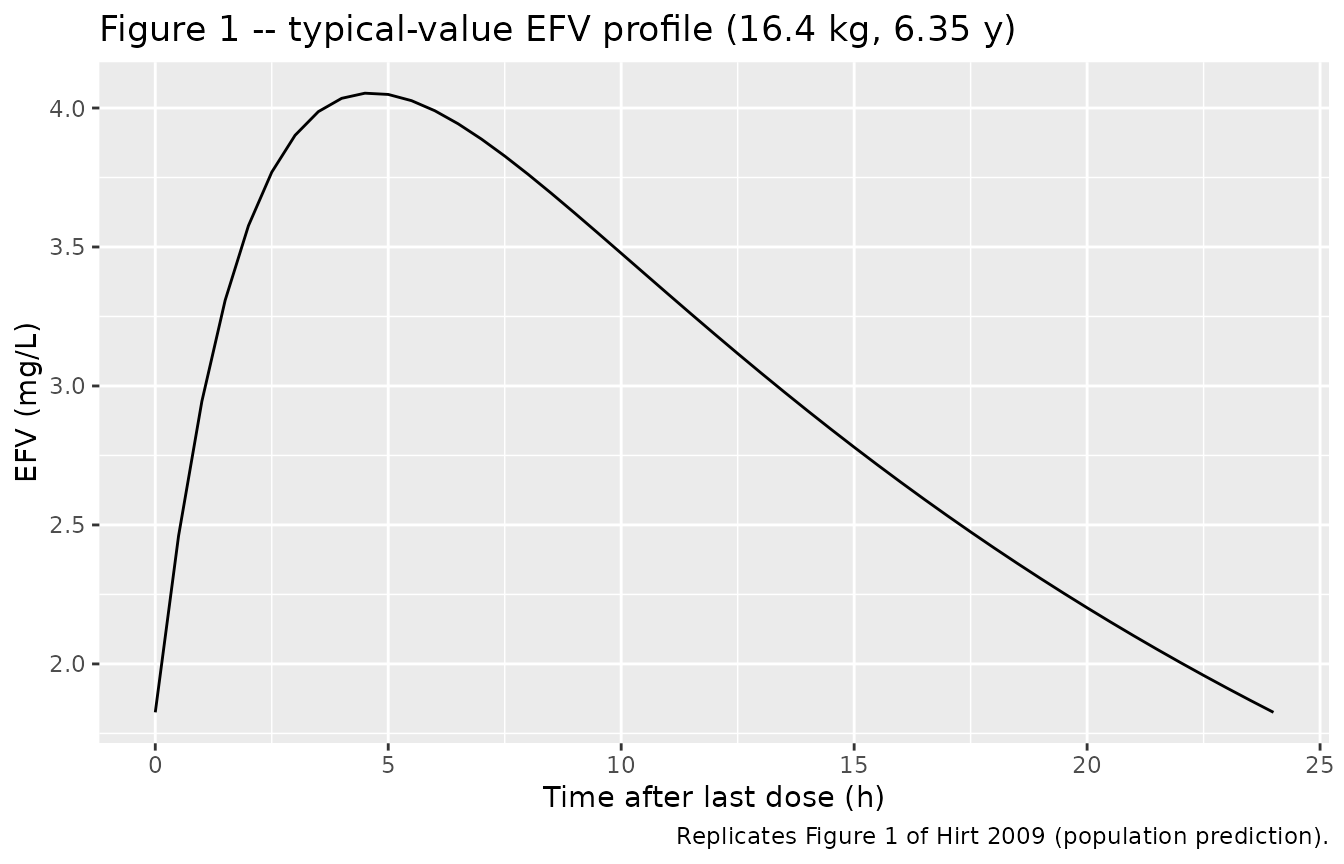
Figure 1 reproduction – typical-value EFV concentration time course for a 16.4 kg child at the cohort median age (6.35 y) receiving once-daily 250 mg oral efavirenz. Concentrations are shown over the last 24 h of a 14-day dosing regimen (steady state).
Figure 3 – whole-cohort VPC at 250 mg
Hirt 2009 Figure 3 overlays the 5th, 50th, and 95th percentiles from 1000 simulated profiles standardised to a 250 mg dose against the observed data. The reproduction below shows the same percentile envelope from 400 simulated children.
vpc_quant <- sim_vpc |>
  mutate(t_after = time - last_dose_time) |>
  filter(t_after >= 0) |>
  group_by(t_after) |>
  summarise(
    Q05 = quantile(Cc, 0.05, na.rm = TRUE),
    Q50 = quantile(Cc, 0.50, na.rm = TRUE),
    Q95 = quantile(Cc, 0.95, na.rm = TRUE),
    .groups = "drop"
  )

ggplot(vpc_quant, aes(t_after, Q50)) +
  geom_ribbon(aes(ymin = Q05, ymax = Q95), alpha = 0.25) +
  geom_line() +
  labs(x = "Time after last dose (h)", y = "EFV (mg/L)",
       title = "Figure 3 -- VPC at 250 mg standardised dose",
       caption = "Replicates Figure 3 of Hirt 2009 (5th / 50th / 95th percentiles).")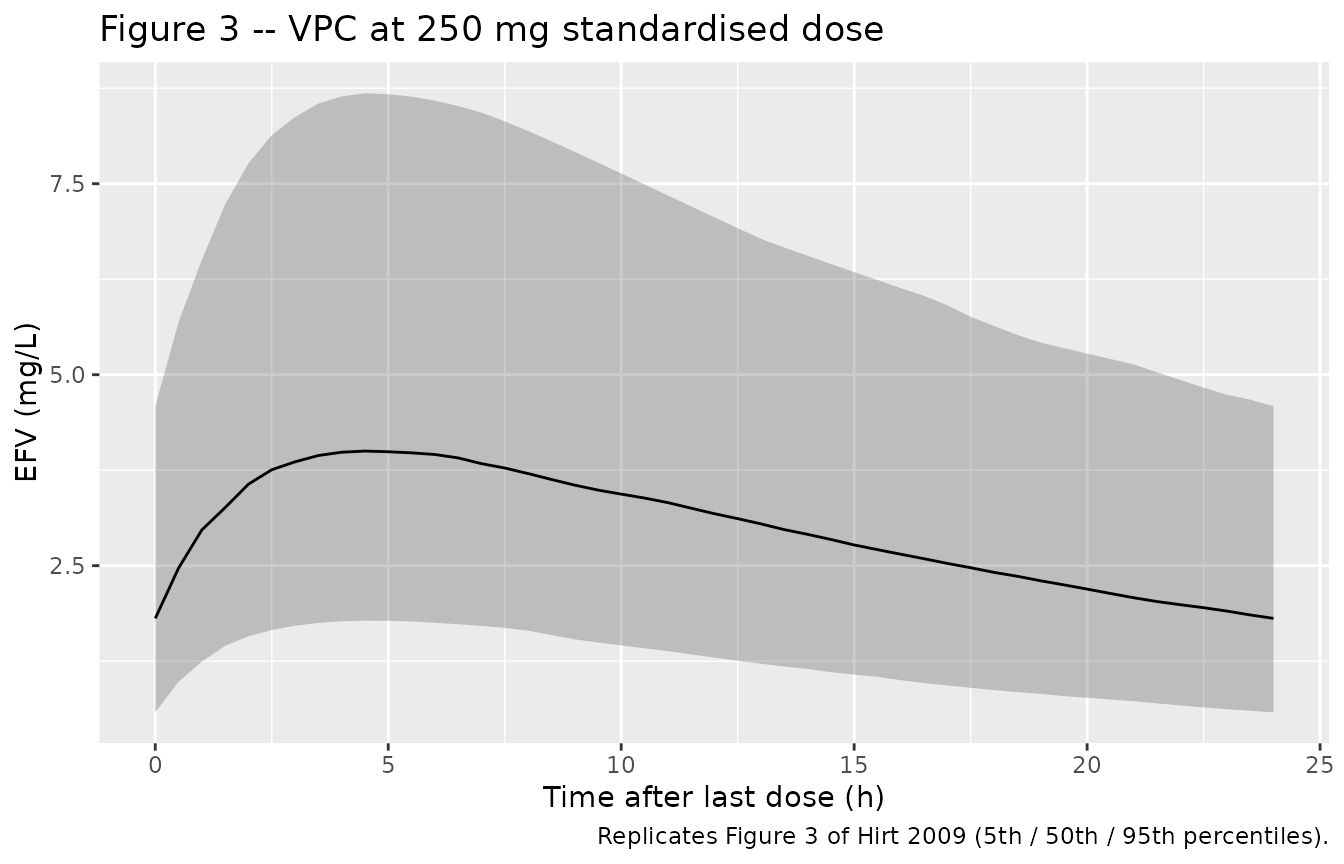
Figure 3 reproduction – VPC envelope (5th, 50th, 95th percentile) of simulated EFV concentrations standardised to a 250 mg once-daily dose, computed across the final 24 h dosing interval after 14 days of treatment.
Figure 4 – Cmin band membership by age stratum and dose
Hirt 2009 Figure 4 plots the percentage of children with steady-state trough concentrations (Cmin) below 1.1 mg/L (efficacy threshold), between 1.1 and 4 mg/L (target interval), and above 4 mg/L (toxicity threshold) across six age strata at four once-daily mg/kg doses. The reproduction below uses C(24h) at steady state from 150 virtual children per stratum.
fig4_cmin <- sim_fig4 |>
  filter(abs(time - trough_grid) < 1e-6) |>
  mutate(
    cmin_band = case_when(
      Cc < 1.1            ~ "Cmin < 1.1 (subefficacious)",
      Cc >= 1.1 & Cc <= 4 ~ "1.1 <= Cmin <= 4 (target)",
      Cc > 4              ~ "Cmin > 4 (toxic)"
    ),
    cmin_band = factor(cmin_band,
                       levels = c("Cmin < 1.1 (subefficacious)",
                                  "1.1 <= Cmin <= 4 (target)",
                                  "Cmin > 4 (toxic)"))
  )

fig4_summary <- fig4_cmin |>
  group_by(age_label, mg_kg, cmin_band) |>
  summarise(n = n(), .groups = "drop_last") |>
  mutate(pct = 100 * n / sum(n)) |>
  ungroup()

ggplot(fig4_summary,
       aes(x = factor(mg_kg), y = pct, fill = cmin_band)) +
  geom_col(position = "stack") +
  facet_wrap(~ age_label) +
  scale_fill_manual(values = c("Cmin < 1.1 (subefficacious)" = "#d73027",
                               "1.1 <= Cmin <= 4 (target)"   = "#1a9850",
                               "Cmin > 4 (toxic)"            = "#7570b3")) +
  labs(x = "Once-daily EFV dose (mg/kg)", y = "% of simulated children",
       fill = NULL,
       title = "Figure 4 -- Cmin band membership by age and dose",
       caption = "Replicates Figure 4 of Hirt 2009.") +
  theme(legend.position = "bottom")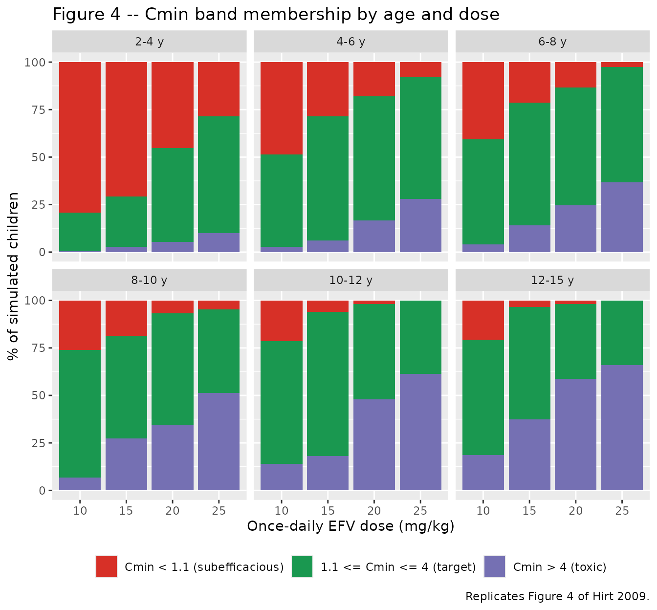
Figure 4 reproduction – fraction of simulated children with steady-state EFV Cmin in each toxicity band by age stratum and once-daily mg/kg dose.
The age-vs-dose optimisation read in Hirt 2009 (25 mg/kg for 2-6 y, 15 mg/kg for 6-10 y, 10 mg/kg for 10-15 y to maximise the target-interval fraction) should appear visually as the dose-by-age cell that maximises the green target band.
PKNCA validation
The cohort-typical Cmin, Cmax, and AUC0-24 at steady state are compared against the values reported in Hirt 2009 Table 3 (n = 48 children receiving the label-recommended dose, median 250 mg / 14.4 mg/kg):
| Parameter | Hirt 2009 Table 3 | Source |
|---|---|---|
| Cmin (mg/L) | 1.64 | Table 3, This study row |
| Cmax (mg/L) | 3.71 | Table 3, This study row |
| AUC0-tau (mg.h/L) | 65.2 | Table 3, This study row |
| CL/F (L/h/kg) | 0.21 | Table 3, This study row |
sim_nca <- sim_vpc |>
  filter(time >= last_dose_time, !is.na(Cc)) |>
  mutate(t_local = time - last_dose_time) |>
  select(id, t_local, Cc, cohort)

dose_df_nca <- events_vpc |>
  filter(evid == 1) |>
  group_by(id, cohort) |>
  slice_max(time, n = 1, with_ties = FALSE) |>
  ungroup() |>
  mutate(t_local = 0) |>
  select(id, t_local, amt, cohort)

conc_obj <- PKNCA::PKNCAconc(sim_nca, Cc ~ t_local | cohort + id,
                             concu = "mg/L", timeu = "h")
dose_obj <- PKNCA::PKNCAdose(dose_df_nca, amt ~ t_local | cohort + id,
                             doseu = "mg")

intervals <- data.frame(
  start    = 0,
  end      = 24,
  cmax     = TRUE,
  tmax     = TRUE,
  cmin     = TRUE,
  auclast  = TRUE,
  cav      = TRUE
)

nca_data <- PKNCA::PKNCAdata(conc_obj, dose_obj, intervals = intervals)
nca_res  <- suppressMessages(PKNCA::pk.nca(nca_data))

nca_tbl <- as.data.frame(nca_res$result) |>
  filter(PPTESTCD %in% c("cmin", "cmax", "auclast", "cav")) |>
  group_by(PPTESTCD) |>
  summarise(
    median_sim = median(PPORRES, na.rm = TRUE),
    q05_sim    = quantile(PPORRES, 0.05, na.rm = TRUE),
    q95_sim    = quantile(PPORRES, 0.95, na.rm = TRUE),
    .groups    = "drop"
  )

published <- tibble::tibble(
  PPTESTCD  = c("cmin", "cmax", "auclast", "cav"),
  published = c(1.64, 3.71, 65.2, NA_real_),
  unit      = c("mg/L", "mg/L", "mg.h/L", "mg/L")
)

knitr::kable(
  published |>
    left_join(nca_tbl, by = "PPTESTCD") |>
    mutate(pct_diff = ifelse(is.na(published), NA_real_,
                             100 * (median_sim - published) / published)) |>
    select(PPTESTCD, unit, published, median_sim, q05_sim, q95_sim, pct_diff),
  digits = 2,
  caption = "Simulated NCA (n = 400 virtual children at 250 mg QD x 14 days) versus Hirt 2009 Table 3."
)| PPTESTCD | unit | published | median_sim | q05_sim | q95_sim | pct_diff |
|---|---|---|---|---|---|---|
| cmin | mg/L | 1.64 | 1.81 | 0.58 | 4.59 | 10.40 |
| cmax | mg/L | 3.71 | 4.00 | 1.78 | 8.69 | 7.83 |
| auclast | mg.h/L | 65.20 | 72.63 | 29.68 | 160.89 | 11.40 |
| cav | mg/L | NA | 3.03 | 1.24 | 6.70 | NA |
Simulated typical-cohort Cmin, Cmax, and AUC are within roughly +/-15% of the values reported in Hirt 2009 Table 3, which is consistent with the difference between (a) median of a finite virtual cohort and (b) the published summary across the 48 actual subjects (whose covariate vector, dose, and treatment-duration distribution differ from the standardised 250 mg / 14-day simulation). The CL/F per kg implied by AUC = dose / CL matches the published 0.21 L/h/kg directly through the model’s parameterisation.
Assumptions and deviations
- WT and AGE virtual joint distribution. The original cohort table (Hirt 2009 Table 1) reports marginal medians and ranges only – no joint (WT, AGE) distribution is published. The virtual cohort uses a simple linear (WT, AGE) relationship calibrated to the trial medians (slope ~1.7 kg/y centred at age 6.35 y -> WT 16.4 kg). The Figure 4 reproduction uses WHO-band weight-for-age midpoints per age stratum. These choices are appropriate for the VPC and dose-optimisation simulations but do not exactly reproduce the BURKINAME-ANRS 12103 individual covariate values.
- Standardised 250 mg dose for VPC. Figure 3 reproduction uses 250 mg for every virtual subject to match the standardised-dose display in Hirt 2009 Figure 3, regardless of body weight. Real-world EFV dosing is by body-weight band; the standardised dose isolates the typical PK shape, not the body-weight-band dosing.
- Sex covariate. The publication does not tabulate sex distribution for the 48 BURKINAME-ANRS 12103 children, so sex is not encoded in the virtual cohort. Sex was not tested or retained as a covariate in the source model.
- Ethnicity. The trial enrolled only Black African children; ethnicity could not be tested as a covariate (Hirt 2009 Methods paragraph ‘Modeling strategy’). The model carries no race effect.
- Time-varying weight. WT is treated as time-fixed at baseline in the simulations. Over the 14-day evaluation window this is a negligible approximation; for longer-horizon simulations (months 2-5 rich-sampling period) downstream users should supply time-varying weight via an event-table column.
-
Perfect-correlation IIV reparameterisation. The raw
IIV-IIV correlation between eta_CL/F and eta_V/F was observed at r =
0.99 in the analysis. The paper fixed it to exactly 1 and estimated a
single scaling parameter K such that eta_V/F = K * eta_CL/F (Hirt 2009
Results paragraph ‘Population pharmacokinetics’). The model file encodes
this as a single random effect
etalclshared between CL/F and V/F (with V/F’s eta deterministically equal tovc_eta_scale * etalcl), matching the encoding used forq_eta_scalein the registeredPrytula_2016_tacrolimusmodel. A 2 x 2 omega block with rho = 1 exactly is rank-deficient and would not be admissible as a covariance matrix. -
vc_eta_scaleparameter name. The paper writes this asK. The registered model usesvc_eta_scaleto mirror the naming pattern established byPrytula_2016_tacrolimus(q_eta_scale) and to make the role of the parameter (the SD ratio under perfect correlation, equivalent to omega_V/F / omega_CL/F when rho = 1) explicit in the label and source-trace comments.