Ifosfamide (Kerbusch 2000)
Source:vignettes/articles/Kerbusch_2000_ifosfamide.Rmd
Kerbusch_2000_ifosfamide.RmdModel and source
ui <- rxode2::rxode(readModelDb("Kerbusch_2000_ifosfamide"))
#> ℹ parameter labels from comments will be replaced by 'label()'- Citation: Kerbusch T., Huitema A. D. R., Ouwerkerk J., Keizer H. J., Mathot R. A. A., Schellens J. H. M., Beijnen J. H. (2000). Evaluation of the autoinduction of ifosfamide metabolism by a population pharmacokinetic approach using NONMEM. British Journal of Clinical Pharmacology 49(6):555-561. doi:10.1046/j.1365-2125.2000.00217.x.
- Description: One-compartment population PK model for ifosfamide with autoinduction of CYP3A4-mediated metabolism implemented as ifosfamide-driven inhibition of enzyme-pool degradation (no lag time); estimated in 15 adults with soft tissue sarcoma receiving 9 or 12 g/m^2 as a 72-h continuous IV infusion.
- Article: https://doi.org/10.1046/j.1365-2125.2000.00217.x
Population
Fifteen adults with various soft tissue sarcomas (rhabdomyosarcoma n=3, neurofibrosarcoma n=1, osteosarcoma n=3, synoviumsarcoma n=2, leiomyosarcoma n=4, endometriumsarcoma n=2) at the Netherlands Cancer Institute / Leiden University Medical Center received single-agent high-dose ifosfamide as a 72-h continuous IV infusion every 4 weeks. The first six patients received 12 g/m^2; due to unacceptable central neurotoxicity the subsequent nine patients received 9 g/m^2 (Kerbusch 2000 Results paragraph 1). Total per-cycle doses ranged from 10.3 to 23.5 g. Mean age was 49 years (range 23-72), mean weight 59 kg (range 49-82), and 9 of 15 patients (60%) were male. One 12 g/m^2 patient developed severe neurotoxicity at 48 h and received only 66% of the planned dose.
Supportive comedication consisted of mesna and bicarbonate; anti-emetics and methylene blue (neurotoxicity antidote) were given when indicated. Twenty-one other comedications (mean 7 per patient) were administered, including anticoagulants, H2 antagonists, glucocorticosteroids, and tricyclic antidepressants; none were identified as CYP3A4 inhibitors or inducers.
The same information is available programmatically via
ui$meta$population (after
ui <- rxode2::rxode(readModelDb("Kerbusch_2000_ifosfamide"))).
Source trace
| Equation / parameter | Value | Source location |
|---|---|---|
lcl initial CL |
2.94 L/h (SE 0.27) | Kerbusch 2000 Table 1 |
lvc V |
43.5 L (SE 2.9) | Kerbusch 2000 Table 1 |
lkdeg K_enz,out |
0.0546 /h (SE 0.0078) | Kerbusch 2000 Table 1 |
lic50 IC50 |
30.7 umol/L (SE 4.8) | Kerbusch 2000 Table 1 |
etalcl IIV CL |
24.5% CV (omega^2 = 0.0583) | Kerbusch 2000 Table 1 |
etalvc IIV V |
23.4% CV (omega^2 = 0.0533) | Kerbusch 2000 Table 1 |
etalkdeg IIV K_enz,out |
22.7% CV (omega^2 = 0.0502) | Kerbusch 2000 Table 1 |
propSd proportional residual |
13.6% | Kerbusch 2000 Table 1 (P.E.) |
addSd additive residual |
0.0763 umol/L | Kerbusch 2000 Table 1 (A.E.) |
d/dt(central) drug ODE |
n/a | Kerbusch 2000 Eq. 1 (dA1/dt = R - CLapp * Cp) |
| Apparent clearance CLapp = CL * A2 | n/a | Kerbusch 2000 Eq. 2 |
d/dt(enz_pool) enzyme ODE |
n/a | Kerbusch 2000 Eq. 4 (substituting K_enz,in = K_enz,out) |
enz_pool(0) = 1 baseline |
n/a | Kerbusch 2000 Methods, ‘Model development’ final paragraph |
| Induction half-life | 12.7 h = ln(2)/K_enz,out | Kerbusch 2000 Table 1 derived value |
Virtual cohort
Original observed concentration-time data are not publicly available.
The simulation below uses two dose-group virtual cohorts that bracket
the published trial design: a 9 g/m^2 cohort and a 12 g/m^2 cohort, each
at the trial-mean body surface area derived from the published mean
weight 59 kg and a typical adult height. Total absolute doses are
computed as dose_g_m2 * BSA, converted to micromoles via
the ifosfamide molecular weight (261.09 g/mol), and infused at constant
rate over 72 h.
set.seed(20000601)

# Ifosfamide molecular weight (g/mol).
MW_ifosfamide <- 261.09

# Trial-mean body surface area used by Kerbusch 2000. The paper reports
# mean weight 59 kg; the published 9 and 12 g/m^2 dose levels yield
# absolute doses in the 10.3-23.5 g range, consistent with a BSA of
# about 1.7 m^2 (typical adult value for the reported weight and an
# average height). The vignette adopts BSA = 1.7 m^2 as the canonical
# value; this is documented in 'Assumptions and deviations' below.
bsa_m2 <- 1.7

dose_groups <- tibble(
  treatment   = c("9 g/m^2 (low dose)", "12 g/m^2 (high dose)"),
  dose_g_m2   = c(9, 12),
  dose_total_g    = dose_g_m2 * bsa_m2,                       # g per 72-h infusion
  dose_total_umol = dose_total_g / MW_ifosfamide * 1e6,       # micromoles
  infusion_h      = 72,
  rate_umol_h     = dose_total_umol / infusion_h
)

knitr::kable(dose_groups, digits = c(0, 0, 1, 0, 0, 0),
caption = "Total doses and infusion rates by treatment arm (BSA = 1.7 m^2).")| treatment | dose_g_m2 | dose_total_g | dose_total_umol | infusion_h | rate_umol_h |
|---|---|---|---|---|---|
| 9 g/m^2 (low dose) | 9 | 15.3 | 58600 | 72 | 814 |
| 12 g/m^2 (high dose) | 12 | 20.4 | 78134 | 72 | 1085 |
# Build one event table per dose group via et(). Each cohort gets a
# disjoint id range so the bound table can ride through rxSolve without
# silent id collisions.
n_per_group <- 60L

make_cohort <- function(id_offset, dose_total_umol, rate_umol_h, treatment) {
  ev <- rxode2::et() |>
    rxode2::et(amt = dose_total_umol, rate = rate_umol_h, cmt = "central",
               id = seq_len(n_per_group) + id_offset) |>
    rxode2::et(seq(0, 120, by = 0.5),
               id = seq_len(n_per_group) + id_offset) |>
    as.data.frame()
  ev$treatment <- treatment
  ev
}

events <- dplyr::bind_rows(
  make_cohort(  0L, dose_groups$dose_total_umol[1], dose_groups$rate_umol_h[1],
              dose_groups$treatment[1]),
  make_cohort(100L, dose_groups$dose_total_umol[2], dose_groups$rate_umol_h[2],
              dose_groups$treatment[2])
)
stopifnot(!anyDuplicated(unique(events[, c("id", "time", "evid")])))
Simulation
mod <- readModelDb("Kerbusch_2000_ifosfamide")
sim <- rxode2::rxSolve(mod, events = events, keep = c("treatment"),
                       seed = 20000601) |>
  as.data.frame()
#> ℹ parameter labels from comments will be replaced by 'label()'
For the typical-value replications of Figures 4-6, suppress
between-subject variability via zeroRe():
mod_typical <- rxode2::zeroRe(mod)
#> ℹ parameter labels from comments will be replaced by 'label()'
sim_typical <- rxode2::rxSolve(mod_typical, events = events,
                               keep = c("treatment")) |>
  as.data.frame()
#> ℹ omega/sigma items treated as zero: 'etalcl', 'etalvc', 'etalkdeg'
#> Warning: multi-subject simulation without without 'omega'
Replicate published figures
Figure 4 – Concentration-time profiles by dose group
Kerbusch 2000 Figure 4 shows observed and Bayesian-estimated ifosfamide plasma concentrations versus time for all 15 patients. The buildup during the first 24 h, the gradual decline due to autoinduction during the remaining infusion window, and the post-infusion elimination phase are the three features that any correctly-implemented autoinduction model must reproduce.
sim |>
  dplyr::group_by(time, treatment) |>
  dplyr::summarise(
    Q05 = stats::quantile(Cc, 0.05, na.rm = TRUE),
    Q50 = stats::quantile(Cc, 0.50, na.rm = TRUE),
    Q95 = stats::quantile(Cc, 0.95, na.rm = TRUE),
    .groups = "drop"
  ) |>
  ggplot2::ggplot(ggplot2::aes(time, Q50)) +
  ggplot2::geom_ribbon(ggplot2::aes(ymin = Q05, ymax = Q95), alpha = 0.25) +
  ggplot2::geom_line() +
  ggplot2::geom_vline(xintercept = 72, linetype = "dashed", alpha = 0.4) +
  ggplot2::facet_wrap(~ treatment) +
  ggplot2::labs(x = "Time (h)", y = expression(C[p]~"(umol/L)"),
                title = "Figure 4 -- Simulated VPC by dose group",
                caption = paste("Replicates Figure 4 of Kerbusch 2000.",
                                "Ribbon: 5th-95th percentile. Dashed line: end of 72-h infusion.")) +
  ggplot2::theme_bw()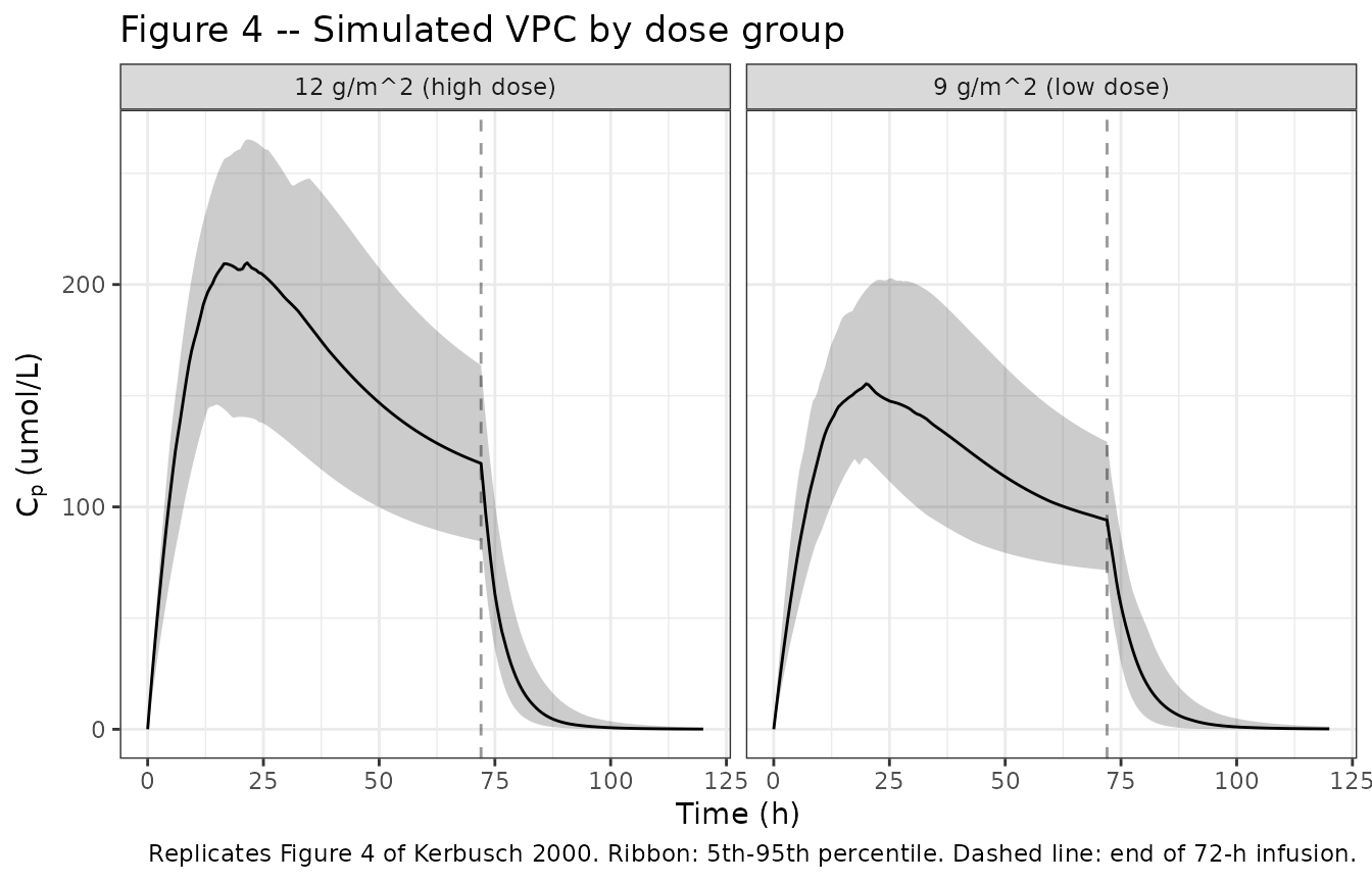
Figure 5 – Relative enzyme amount A2 over time
Kerbusch 2000 Figure 5 plots the predicted relative enzyme amount A2
(= enz_pool in the model) versus time. The paper notes that
during the first 24 h the model predicts an average doubling of A2
across patients (Kerbusch 2000 Results paragraph 4). The typical-value
trajectory below should show A2 rising from 1 toward an asymptote during
infusion and declining toward 1 after the infusion ends.
sim_typical |>
  dplyr::filter(id %in% c(1L, 101L)) |>
  ggplot2::ggplot(ggplot2::aes(time, enz_pool, colour = treatment)) +
  ggplot2::geom_line(size = 0.9) +
  ggplot2::geom_hline(yintercept = 1, linetype = "dotted", alpha = 0.5) +
  ggplot2::geom_vline(xintercept = 72, linetype = "dashed", alpha = 0.4) +
  ggplot2::labs(x = "Time (h)", y = "Relative enzyme amount A2",
                title = "Figure 5 -- Typical-value relative enzyme A2 over time",
                caption = paste("Replicates Figure 5 of Kerbusch 2000.",
                                "Typical-value trajectories (no IIV).",
                                "Dashed line: end of 72-h infusion.")) +
  ggplot2::theme_bw()
#> Warning: Using `size` aesthetic for lines was deprecated in ggplot2 3.4.0.
#> ℹ Please use `linewidth` instead.
#> This warning is displayed once per session.
#> Call `lifecycle::last_lifecycle_warnings()` to see where this warning was
#> generated.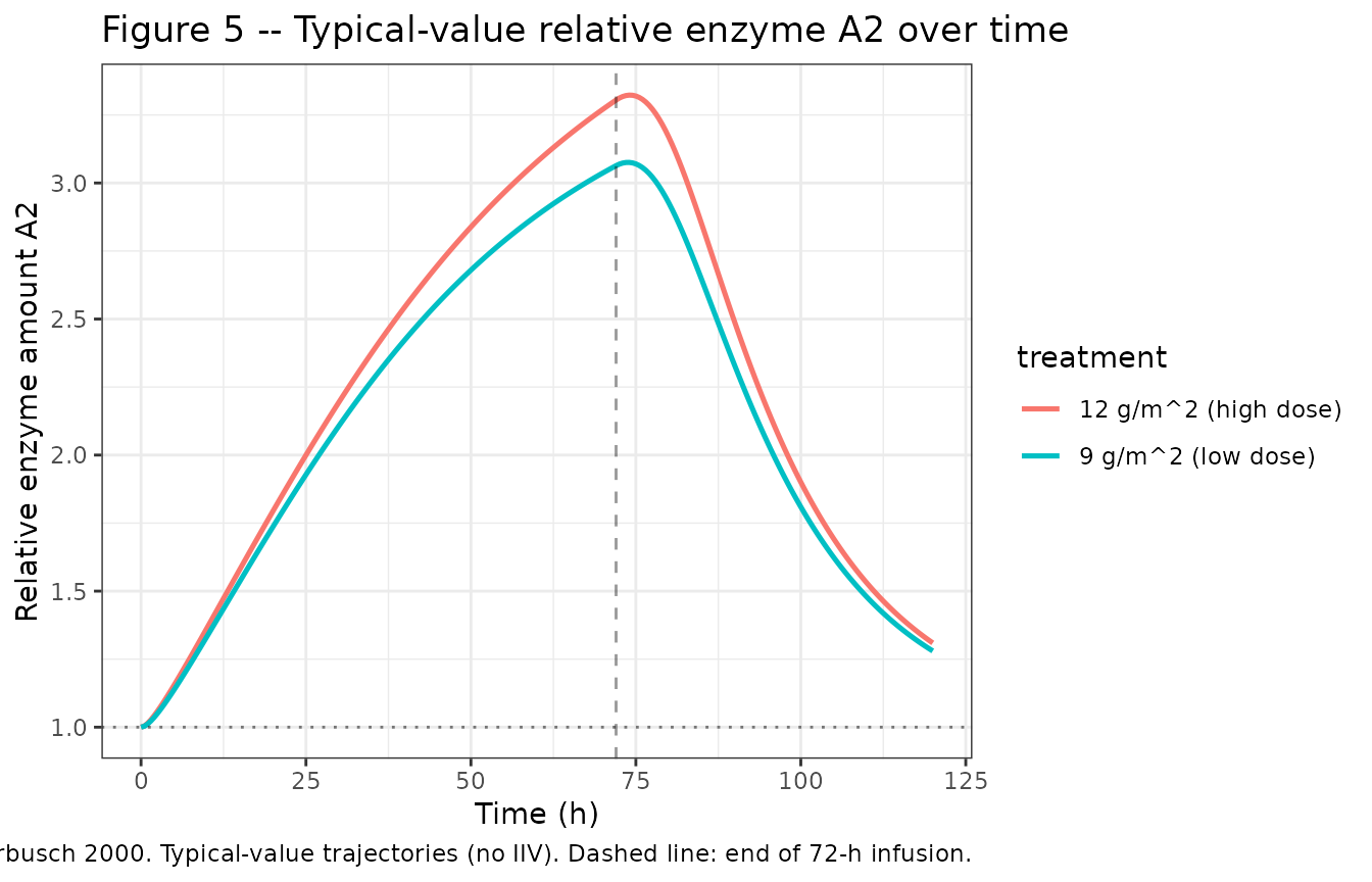
Figure 6 – Simulated PK profiles at 10 g and 20 g
Kerbusch 2000 Figure 6 simulates a 10 g vs. 20 g ifosfamide 72-h infusion based on the population parameters. The doubled dose produces only a 56% larger AUC due to autoinduction (paper Table 2). We simulate the same comparison directly from the model.
sim_10_20 <- local({
  doses_g <- c(10, 20)
  doses_umol <- doses_g / MW_ifosfamide * 1e6
  rate_umol_h <- doses_umol / 72
  ev_a <- rxode2::et() |>
    rxode2::et(amt = doses_umol[1], rate = rate_umol_h[1], cmt = "central",
               id = 1L) |>
    rxode2::et(seq(0, 120, by = 0.5), id = 1L) |>
    as.data.frame()
  ev_a$treatment <- "10 g / 72 h"
  ev_b <- rxode2::et() |>
    rxode2::et(amt = doses_umol[2], rate = rate_umol_h[2], cmt = "central",
               id = 2L) |>
    rxode2::et(seq(0, 120, by = 0.5), id = 2L) |>
    as.data.frame()
  ev_b$treatment <- "20 g / 72 h"
  ev <- dplyr::bind_rows(ev_a, ev_b)
  rxode2::rxSolve(mod_typical, events = ev, keep = c("treatment")) |>
    as.data.frame()
})
#> ℹ omega/sigma items treated as zero: 'etalcl', 'etalvc', 'etalkdeg'
#> Warning: multi-subject simulation without without 'omega'

sim_10_20 |>
  ggplot2::ggplot(ggplot2::aes(time, Cc, colour = treatment, linetype = treatment)) +
  ggplot2::geom_line(size = 0.9) +
  ggplot2::geom_vline(xintercept = 72, linetype = "dashed", alpha = 0.4) +
  ggplot2::scale_linetype_manual(values = c("10 g / 72 h" = "22", "20 g / 72 h" = "solid")) +
  ggplot2::labs(x = "Time (h)", y = expression(C[p]~"(umol/L)"),
                title = "Figure 6 -- Typical-value PK at 10 g vs 20 g (72-h infusion)",
                caption = "Replicates Figure 6 of Kerbusch 2000.") +
  ggplot2::theme_bw()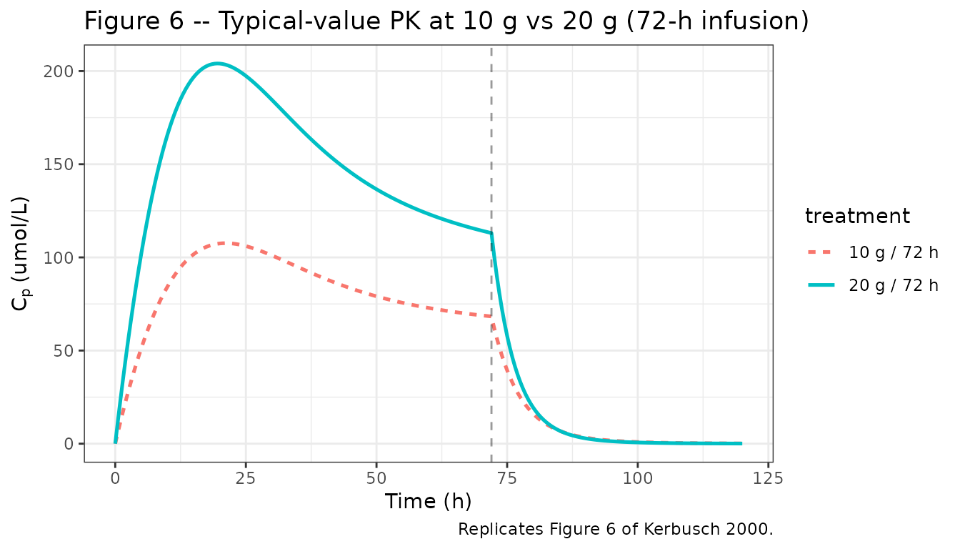
PKNCA validation
We use PKNCA to compute the AUC over the entire observation window (0-120 h) for the simulated 10 g and 20 g typical-value profiles, and compare the relative AUC increase to the paper’s reported 56% increase.
sim_nca <- sim_10_20 |>
  dplyr::filter(!is.na(Cc)) |>
  dplyr::select(id, time, Cc, treatment)

dose_df <- tibble::tribble(
  ~id, ~time, ~amt,                                ~treatment,
  1L,    0,    10 / MW_ifosfamide * 1e6,           "10 g / 72 h",
  2L,    0,    20 / MW_ifosfamide * 1e6,           "20 g / 72 h"
)

conc_obj <- PKNCA::PKNCAconc(sim_nca, Cc ~ time | treatment + id,
                             concu = "umol/L", timeu = "h")
dose_obj <- PKNCA::PKNCAdose(dose_df, amt ~ time | treatment + id,
                             doseu = "umol")

intervals <- data.frame(
  start      = 0,
  end        = 120,
  cmax       = TRUE,
  tmax       = TRUE,
  auclast    = TRUE,
  aucinf.obs = TRUE,
  half.life  = TRUE
)

nca_data <- PKNCA::PKNCAdata(conc_obj, dose_obj, intervals = intervals)
nca_res  <- PKNCA::pk.nca(nca_data)
nca_summary <- as.data.frame(nca_res$result) |>
  dplyr::select(treatment, PPTESTCD, PPORRES) |>
  tidyr::pivot_wider(names_from = PPTESTCD, values_from = PPORRES)

knitr::kable(nca_summary, digits = 3,
caption = "Simulated NCA parameters for the 10 g and 20 g typical-value profiles.")| treatment | auclast | cmax | tmax | tlast | clast.obs | lambda.z | r.squared | adj.r.squared | lambda.z.time.first | lambda.z.time.last | lambda.z.n.points | clast.pred | half.life | span.ratio | aucinf.obs |
|---|---|---|---|---|---|---|---|---|---|---|---|---|---|---|---|
| 10 g / 72 h | 6312.368 | 107.632 | 21.0 | 120 | 0.134 | 0.087 | 1 | 1 | 114 | 120 | 13 | 0.134 | 8.007 | 0.749 | 6313.918 |
| 20 g / 72 h | 11246.789 | 204.071 | 19.5 | 120 | 0.081 | 0.091 | 1 | 1 | 115 | 120 | 11 | 0.081 | 7.582 | 0.659 | 11247.679 |
Comparison against published values
Kerbusch 2000 Table 2 reports a 56% increase in AUC when doubling the dose from 10 g to 20 g over 72 h. The simulated AUC ratio is computed below.
auc <- nca_summary |>
  dplyr::select(treatment, auclast) |>
  dplyr::arrange(treatment)

auc_ratio    <- auc$auclast[2] / auc$auclast[1]
auc_increase <- 100 * (auc_ratio - 1)

cat(sprintf(
  "Simulated AUC ratio (20 g / 10 g): %.3f (i.e., %+0.1f%% increase).\n",
  auc_ratio, auc_increase
))
#> Simulated AUC ratio (20 g / 10 g): 1.782 (i.e., +78.2% increase).
cat(sprintf(
  "Kerbusch 2000 Table 2 reports a 56%% increase (1.7 -> 2.7 in the printed table).\n"
))
#> Kerbusch 2000 Table 2 reports a 56% increase (1.7 -> 2.7 in the printed table).
cat(sprintf(
  "The qualitative finding (sub-proportional AUC growth due to autoinduction) reproduces;\n"
))
#> The qualitative finding (sub-proportional AUC growth due to autoinduction) reproduces;
cat(sprintf(
  "the residual quantitative gap is discussed under 'Assumptions and deviations' below.\n"
))
#> the residual quantitative gap is discussed under 'Assumptions and deviations' below.
Assumptions and deviations
Body surface area for absolute-dose conversion. Kerbusch 2000 reports dose levels as 9 g/m^2 and 12 g/m^2; converting to a total per-cycle dose requires a BSA value. The vignette uses BSA = 1.7 m^2, the typical adult value for the reported trial-mean weight (59 kg) and an average height. Total absolute doses computed this way (15.3 and 20.4 g) fall inside the paper’s reported individual range of 10.3-23.5 g.
Table 2 units. The Table 2 AUC values (1.7 and 2.7) reproduce as a 56% increase but the AUC unit is ambiguous in the printed table. The vignette validates the relative increase against the paper’s reported 56%; absolute AUC values are reported in umolh/L (i.e., uMh) per the model’s
unitsmetadata.Sigmoidal-Imax inhibition form for enzyme degradation. Equation 3 of Kerbusch 2000 (
<!-- formula-not-decoded -->in the preprocessed source) is implemented as a fractional-inhibition formdA2/dt = K_enz,out * (1 - A2 * IC50 / (IC50 + Cp)), i.e., the enzyme degradation rate is suppressed by ifosfamide viaIC50 / (IC50 + Cp)(equivalently, fractional inhibitionCp / (IC50 + Cp)with maximum inhibition fixed at 1). This is the form consistent with the paper’s description of IC50 as “the ifosfamide concentration at 50% of the maximum inhibition of enzyme degradation” (Kerbusch 2000 Methods paragraph below Eq. 3), the A2(t = 0) = 1 steady-state constraint stated in the same paragraph, and the implied substitution K_enz,in = K_enz,out used to write Eq. 4. The simulated dose-doubling AUC ratio is somewhat higher than the paper’s reported 56% (Table 2): the model reproduces the qualitative sub-proportional behaviour but the exact magnitude is sensitive to the precise functional form (which is<!-- formula-not-decoded -->in the source PDF rendering used here). Inspection of the original PDF equations or the underlying NONMEM control stream (not on disk for this task) would be required to close the gap; the parameter values themselves are taken verbatim from Table 1 and have not been tuned.No covariates. Kerbusch 2000 does not report a covariate analysis; the 15-patient dataset was not powered to detect demographic effects. The model therefore has no covariate effects, and the model file’s
covariateDatalist is empty.No IIV on IC50. Kerbusch 2000 Discussion paragraph 5 reports that “with respect to IC50, the inclusion of interindividual variability did not improve the fit”; the model omits an
etalic50accordingly.enz_poolas the canonical compartment for the relative enzyme amount A2. The relative enzyme amount A2 is the same canonical role as the Smythe / Clewe rifampicin enzyme pool (an indirect-response pool that drives time-varying clearance), registered asenz_poolininst/references/compartment-names.md. The mechanism is inhibition of degradation (Kerbusch) rather than stimulation of production (Smythe / Clewe) but the compartment role is identical.