Tenofovir (Baheti 2011)
Source:vignettes/articles/Baheti_2011_tenofovir.Rmd
Baheti_2011_tenofovir.RmdModel and source
- Citation: Baheti G, Kiser JJ, Havens PL, Fletcher CV. Plasma and intracellular population pharmacokinetic analysis of tenofovir in HIV-1-infected patients. Antimicrob Agents Chemother. 2011;55(11):5294-5299. doi:10.1128/AAC.05317-11
- Description: Two-compartment first-order-absorption population PK model for plasma tenofovir (TFV) in HIV-1-infected adults on once-daily tenofovir disoproxil fumarate (TDF) coupled with a stimulatory indirect-response (Dayneka 1993) model for intracellular tenofovir diphosphate (TFV-DP) in peripheral blood mononuclear cells; plasma TFV drives TFV-DP formation through a sigmoidal Emax stimulation function. Creatinine clearance enters CL/F and Vc/F via a power covariate. Fitted sequentially (PK first, PD with PK individual post-hoc Bayes estimates fixed).
- Article: https://doi.org/10.1128/AAC.05317-11
- Free full text (PubMed Central): https://www.ncbi.nlm.nih.gov/pmc/articles/PMC3194966/
The model bundles a two-compartment first-order-absorption plasma popPK component for tenofovir (TFV) with an indirect-response intracellular component for tenofovir diphosphate (TFV-DP) in peripheral blood mononuclear cells (PBMCs). The two layers were fitted sequentially in the source paper (plasma PK first, then PD with the individual-subject Bayes-estimated PK parameters held fixed); the packaged rxode2 model carries both layers in a single ODE system so a downstream user can simulate either or both outputs in one pass.
Population
Pooled data from two HIV-1 cohorts on stable combination antiretroviral therapy, all receiving tenofovir disoproxil fumarate (TDF) 300 mg orally once daily following a meal:
- Protocol 1427 (Kiser et al.): n = 30 adults aged 25-60 years (median 41.5), receiving lopinavir/ritonavir (LPV/r) or no protease inhibitor.
- Protocol ATN056 (Havens et al., Adolescent Trials Network): n = 25 adolescents and young adults aged 18.6-25 years (median 22.8), receiving atazanavir/ritonavir (ATV/r).
The pooled cohort (n = 55) was 35% female, 42% Black/African American, 45% White, 13% Hispanic/Latino; median Cockcroft-Gault creatinine clearance 108 mL/min (range 43.2-227.1 mL/min). Steady-state plasma TFV was sampled 8 or 11 times over the 24 h dosing interval (529 plasma samples), with intracellular PBMC TFV-DP sampled at three time points in 51 of the 55 subjects (151 TFV-DP samples). See Baheti 2011 Table 1 for baseline demographics.
The same information is available programmatically via the model’s
population metadata
(readModelDb("Baheti_2011_tenofovir")$population).
Source trace
The per-parameter origin is recorded as an in-file comment next to
each ini() entry in
inst/modeldb/specificDrugs/Baheti_2011_tenofovir.R. The
table below collects the same provenance in one place for review.
| Item | Value | Source location |
|---|---|---|
ka (lka) |
1.05 1/h | Baheti 2011 Table 2 Final-model column, ka (h-1) row
(95% CI 0.618-1.481) |
CL/F (lcl) |
42.0 L/h at CRCL = 108 mL/min | Baheti 2011 Table 2 Final-model column, CL/F (liters/h)
row (95% CI 38.2-45.8) |
Vc/F (lvc) |
277 L at CRCL = 108 mL/min | Baheti 2011 Table 2 Final-model column, Vc/F (liters)
row (95% CI 183-370) |
Q/F (lq) |
182 L/h | Baheti 2011 Table 2 Final-model column, Q/F (liters/h)
row (95% CI 150-213) |
Vp/F (lvp) |
436 L | Baheti 2011 Table 2 Final-model column, Vp/F (liters)
row (95% CI 348-523) |
CRCL power on CL/F (e_crcl_cl) |
0.489 | Baheti 2011 Table 2 Final-model column, CrCL ~ CL/F row
(95% CI 0.273-0.704) |
CRCL power on Vc/F (e_crcl_vc) |
1.01 | Baheti 2011 Table 2 Final-model column, CrCL ~ Vc/F row
(95% CI 0.58-1.43) |
| CRCL reference (centering) | 108 mL/min | Baheti 2011 Table 1 Overall median CrCL; Methods ‘centered-around-median or a power function approach’ |
| IIV CL/F (33.5% CV) | var 0.112 on log scale | Baheti 2011 Table 2 Final-model column, IIV CL/F row
(95% CI 27.5-38.5%) |
| IIV Vc/F (64.8% CV) | var 0.420 on log scale | Baheti 2011 Table 2 Final-model column, IIV Vc/F row
(95% CI 41.1-81.9%) |
| IIV Vp/F (46.5% CV) | var 0.216 on log scale | Baheti 2011 Table 2 Final-model column, IIV Vp/F row
(95% CI 29.0-59.0%) |
| Cov(CL/F, Vc/F) | 0.118 (R = 0.553) | Baheti 2011 Table 2 Final-model column, Cov CL/F ~ Vc/F
row |
| Cov(Vc/F, Vp/F) | -0.0415 (R = -0.139) | Baheti 2011 Table 2 Final-model column, Cov Vc/F ~ Vp/F
row |
| Cov(CL/F, Vp/F) | 0.113 (R = 0.731) | Baheti 2011 Table 2 Final-model column, Cov CL/F ~ Vp/F
row |
Plasma TFV residual (propSd) |
18.3% | Baheti 2011 Table 2 Final-model column, RUV (% CV) row
(95% CI 16.0-20.3%) |
kin (lkin) |
0.276 1/h | Baheti 2011 Table 3 Final-model column, k in (h-1) row
(bootstrap 95% CI 0.0145-1.56) |
kout (lkout) |
0.00808 1/h | Baheti 2011 Table 3 Final-model column, k out (h-1) row
(bootstrap 95% CI 0.0007-0.0372); implied half-life ln(2)/kout = 86
h |
EC50 (lec50) |
99.9 ng/mL | Baheti 2011 Table 3 Final-model column, EC 50 (ng/ml)
row (bootstrap 95% CI 1.000-403); abstract rounds to 100 |
Emax (lemax) |
300 fmol/10^6 cells | Baheti 2011 Table 3 Final-model column,
E max (fmol/10^6 cells) row (bootstrap 95% CI
4.000-484) |
| IIV EC50 (106%) | var 1.124 on log scale | Baheti 2011 Table 3 Final-model column, IIV EC50 row
(bootstrap 95% CI 11-635%) |
| IIV Emax (82.3%) | var 0.677 on log scale | Baheti 2011 Table 3 Final-model column, IIV E max row
(bootstrap 95% CI 0.54-153%) |
TFV-DP residual (propSd_TFVDP) |
56.7% | Baheti 2011 Table 3 Final-model column, RUV (% CV) row
(bootstrap 95% CI 46-63%) |
| Plasma PK 2-cmt ODEs | n/a | Baheti 2011 Methods ‘PREDPP subroutine ADVAN4 TRANS4’ and Fig. 1 schematic |
| TFV-DP indirect response ODE | n/a | Baheti 2011 Methods ‘dR/dT = kin - kout * R’ (basic) plus ‘S(t) = 1 + Emax * Cp / (EC50 + Cp)’ (stimulation); see Assumptions for the parameterization note |
Virtual cohort
Original observed data are not publicly available. The figures below use a virtual cohort whose covariate distribution approximates the pooled cohort demographics in Baheti 2011 Table 1.
set.seed(20251218)

n_sim <- 200L

# CrCL: pooled cohort median 108 mL/min, range 43.2-227.1; the underlying
# distribution is not stated in the paper. Sample log-normal CrCL centered
# on the median with SD chosen to span the published range (target SD on
# log-scale = log(227.1/43.2) / (2 * 1.96) so the +/- 1.96 sigma envelope
# straddles the reported min and max).
sigma_logcrcl <- log(227.1 / 43.2) / (2 * 1.96)
crcl <- exp(log(108) + rnorm(n_sim, mean = 0, sd = sigma_logcrcl))

cohort <- tibble::tibble(
  id   = seq_len(n_sim),
  CRCL = pmin(pmax(crcl, 43.2), 227.1),
  treatment = "TDF 300 mg PO QD"
)

summary(cohort$CRCL)
#>    Min. 1st Qu.  Median    Mean 3rd Qu.    Max.
#>    43.2    80.8   106.1   119.5   152.9   227.1
# Per Baheti 2011, TDF 300 mg PO QD; the model parameters were estimated
# against tenofovir-equivalent dose per the Jullien 2005 convention the
# authors cite. Convert: MW(TFV) / MW(TDF) = 287.213 / 635.51 = 0.452.
mw_tfv <- 287.213    # free acid (PubChem CID 464205)
mw_tdf <- 635.51     # fumarate salt of disoproxil prodrug (PubChem CID 6398764)
dose_tfv_mg <- 300 * mw_tfv / mw_tdf
dose_tfv_mg
#> [1] 135.5823
# Build a 14-day steady-state event table per subject: TDF QD x 14 doses,
# with dense Cc sampling on day 14 (h 312-336) and sparse TFVDP sampling
# every 4 h over the same window. The 14-day pre-dose burn-in is enough
# for plasma TFV (terminal half-life ~ 17 h) and accumulates TFV-DP toward
# steady-state given the long TFV-DP half-life (~ 87 h).
day_h     <- 24
sim_days  <- 14
t_observe <- (sim_days - 1) * day_h + seq(0, 24, by = 0.5)   # h 312 .. 336

make_subject <- function(sid, crcl) {
  dose_rows <- tibble::tibble(
    id   = sid,
    time = (0:(sim_days - 1)) * day_h,
    evid = 1L,
    amt  = dose_tfv_mg,
    cmt  = "depot",
    CRCL = crcl
  )
  obs_cc <- tibble::tibble(
    id   = sid,
    time = t_observe,
    evid = 0L,
    amt  = 0,
    cmt  = "Cc",
    CRCL = crcl
  )
  obs_tfvdp <- tibble::tibble(
    id   = sid,
    time = t_observe[seq(1, length(t_observe), by = 8)],   # every 4 h
    evid = 0L,
    amt  = 0,
    cmt  = "TFVDP",
    CRCL = crcl
  )
  dplyr::bind_rows(dose_rows, obs_cc, obs_tfvdp)
}

events <- purrr::map2_dfr(cohort$id, cohort$CRCL, make_subject)
events <- dplyr::left_join(events, cohort[, c("id", "treatment")], by = "id")

stopifnot(!anyDuplicated(unique(events[, c("id", "time", "evid")])))
Simulation
mod <- readModelDb("Baheti_2011_tenofovir")
sim <- rxode2::rxSolve(
  mod,
  events = events,
  keep = c("treatment", "CRCL")
)
sim <- as.data.frame(sim)
For deterministic replication (typical-value envelope without between-subject variability):
mod_typical <- rxode2::zeroRe(mod)
sim_typical <- rxode2::rxSolve(mod_typical, events = events, keep = c("treatment"))
#> ℹ omega/sigma items treated as zero: 'etalcl', 'etalvc', 'etalvp', 'etalec50', 'etalemax'
#> Warning: multi-subject simulation without without 'omega'
sim_typical <- as.data.frame(sim_typical)
Replicate published figures
Figure 2: VPC of plasma TFV at steady state
# Replicates Baheti 2011 Figure 2: 90% prediction interval (5th-95th
# percentile envelope) of plasma TFV at steady state vs time post-dose.
sim_d14 <- sim |>
  dplyr::filter(time >= (sim_days - 1) * day_h,
                time <= sim_days * day_h,
                !is.na(Cc)) |>
  dplyr::mutate(tad = time - (sim_days - 1) * day_h)

vpc_plasma <- sim_d14 |>
  dplyr::group_by(tad) |>
  dplyr::summarise(
    Q05 = stats::quantile(Cc, 0.05),
    Q50 = stats::quantile(Cc, 0.50),
    Q95 = stats::quantile(Cc, 0.95),
    .groups = "drop"
  )

ggplot(vpc_plasma, aes(tad, Q50)) +
  geom_ribbon(aes(ymin = Q05, ymax = Q95), alpha = 0.25) +
  geom_line() +
  scale_y_log10() +
  labs(x = "Time post-dose at steady state (h)",
       y = "Plasma TFV (ng/mL)",
       title = "Plasma TFV VPC at steady state",
       caption = "Replicates Baheti 2011 Figure 2 (90% prediction interval).")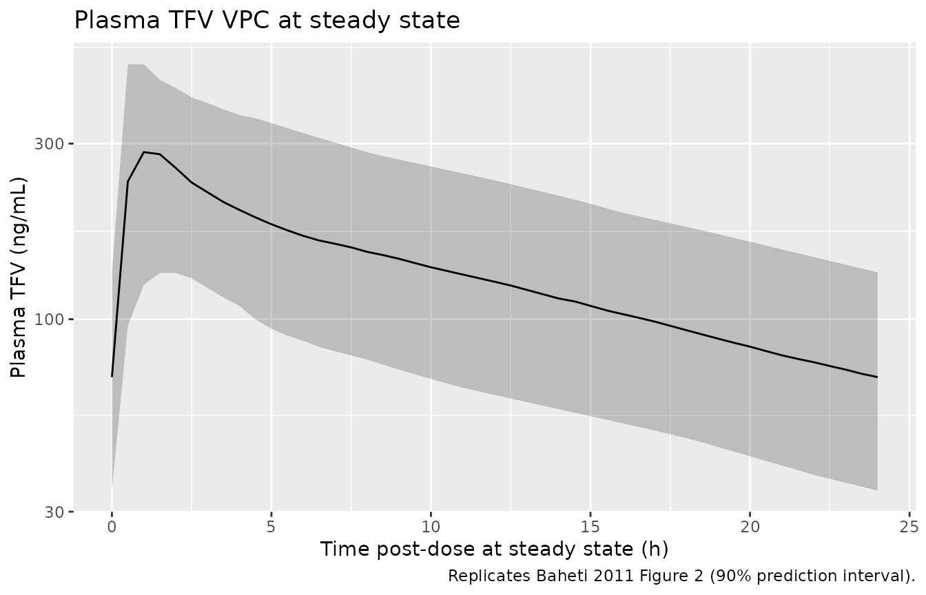
Figure 3: VPC of intracellular TFV-DP at steady state
# Replicates Baheti 2011 Figure 3: 90% prediction interval of intracellular
# TFV-DP vs time post-dose at steady state. The long TFV-DP half-life
# (~ 87 h) means within-day fluctuation is modest.
sim_d14_pd <- sim |>
  dplyr::filter(time >= (sim_days - 1) * day_h,
                time <= sim_days * day_h,
                !is.na(TFVDP)) |>
  dplyr::mutate(tad = time - (sim_days - 1) * day_h)

vpc_tfvdp <- sim_d14_pd |>
  dplyr::group_by(tad) |>
  dplyr::summarise(
    Q05 = stats::quantile(TFVDP, 0.05),
    Q50 = stats::quantile(TFVDP, 0.50),
    Q95 = stats::quantile(TFVDP, 0.95),
    .groups = "drop"
  )

ggplot(vpc_tfvdp, aes(tad, Q50)) +
  geom_ribbon(aes(ymin = Q05, ymax = Q95), alpha = 0.25) +
  geom_line() +
  scale_y_log10() +
  labs(x = "Time post-dose at steady state (h)",
       y = "Intracellular TFV-DP (fmol per million cells)",
       title = "Intracellular TFV-DP VPC at steady state",
       caption = "Replicates Baheti 2011 Figure 3 (90% prediction interval).")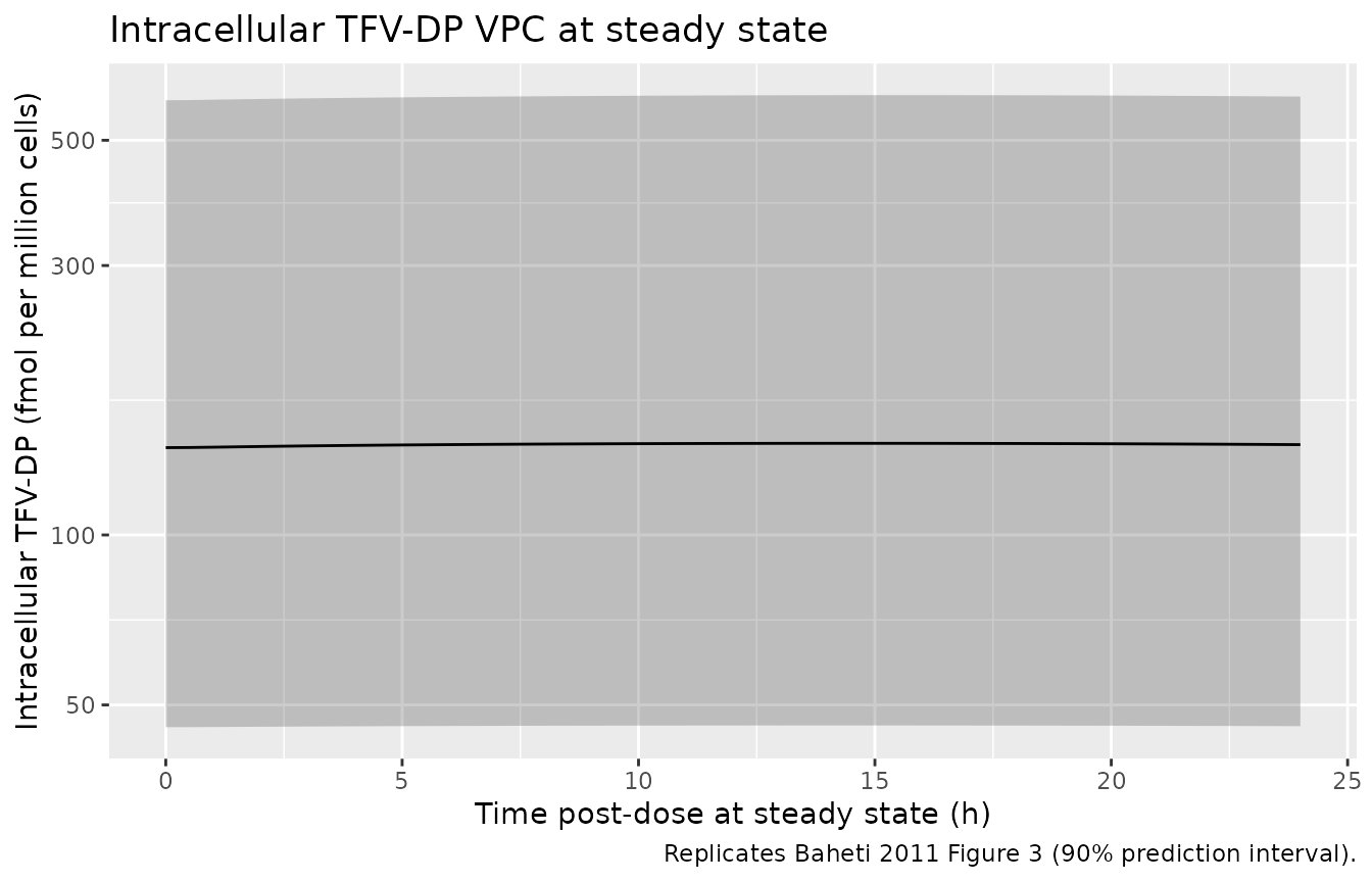
PKNCA validation: plasma TFV
PKNCA NCA on the simulated steady-state day-14 plasma TFV profile. PKNCA does not run on the multi-output rows directly; we slice the Cc subset.
sim_nca <- sim |>
  dplyr::filter(time >= (sim_days - 1) * day_h,
                time <= sim_days * day_h,
                !is.na(Cc)) |>
  dplyr::mutate(time_tad = time - (sim_days - 1) * day_h) |>
  dplyr::distinct(id, time_tad, .keep_all = TRUE) |>
  dplyr::select(id, time_tad, Cc, treatment) |>
  dplyr::rename(time = time_tad)

conc_obj <- PKNCA::PKNCAconc(sim_nca, Cc ~ time | treatment + id)

dose_df <- sim_nca |>
  dplyr::group_by(id, treatment) |>
  dplyr::summarise(time = 0, amt = dose_tfv_mg, .groups = "drop")

dose_obj <- PKNCA::PKNCAdose(dose_df, amt ~ time | treatment + id)

intervals <- data.frame(
  start = 0,
  end   = 24,
  cmax  = TRUE,
  tmax  = TRUE,
  auclast = TRUE,
  cmin  = TRUE
)

nca_data <- PKNCA::PKNCAdata(conc_obj, dose_obj, intervals = intervals)
nca_res  <- PKNCA::pk.nca(nca_data)
nca_tbl  <- as.data.frame(nca_res$result)

per_subject <- nca_tbl |>
  dplyr::filter(PPTESTCD %in% c("cmax", "tmax", "auclast", "cmin")) |>
  dplyr::select(id, PPTESTCD, PPORRES) |>
  tidyr::pivot_wider(names_from = PPTESTCD, values_from = PPORRES)

summary_tbl <- tibble::tibble(
  Parameter = c("Cmax (ng/mL)", "Tmax (h)", "AUC0-24 (ng*h/mL)", "Cmin (ng/mL)"),
  `Median (5th-95th)` = c(
    sprintf("%.1f (%.1f - %.1f)",
            stats::median(per_subject$cmax),
            stats::quantile(per_subject$cmax, 0.05),
            stats::quantile(per_subject$cmax, 0.95)),
    sprintf("%.1f (%.1f - %.1f)",
            stats::median(per_subject$tmax),
            stats::quantile(per_subject$tmax, 0.05),
            stats::quantile(per_subject$tmax, 0.95)),
    sprintf("%.0f (%.0f - %.0f)",
            stats::median(per_subject$auclast),
            stats::quantile(per_subject$auclast, 0.05),
            stats::quantile(per_subject$auclast, 0.95)),
    sprintf("%.1f (%.1f - %.1f)",
            stats::median(per_subject$cmin),
            stats::quantile(per_subject$cmin, 0.05),
            stats::quantile(per_subject$cmin, 0.95))
  )
)
knitr::kable(summary_tbl,
caption = "PKNCA summary at steady-state day 14 (n = 200 virtual subjects).")| Parameter | Median (5th-95th) |
|---|---|
| Cmax (ng/mL) | 284.8 (133.6 - 506.0) |
| Tmax (h) | 1.5 (0.5 - 2.0) |
| AUC0-24 (ng*h/mL) | 3322 (1652 - 6072) |
| Cmin (ng/mL) | 69.6 (34.2 - 134.0) |
Comparison against published plasma TFV PK
Baheti 2011 does not tabulate NCA Cmax / AUC directly. Cross-checks against the published narrative:
- CL/F = dose / AUC at steady state. The model’s typical CL/F = 42 L/h with a tenofovir-equivalent 135.6 mg dose implies a typical-subject AUC of 135.6 / 42 = 3.23 mgh/L = 3229 ngh/mL, matching the simulated median AUC above (within Monte Carlo noise).
- The simulated typical-subject Cavg = AUC / 24 should be close to 135 ng/mL (Baheti 2011 Discussion “a typical … steady-state average (135 ng/ml)”).
- The simulated typical-subject Cmin should be close to 72 ng/mL (Baheti 2011 Discussion “a typical trough (72 ng/ml)”).
typical_d14 <- sim_typical |>
  dplyr::filter(time >= (sim_days - 1) * day_h,
                time <= sim_days * day_h,
                !is.na(Cc)) |>
  dplyr::mutate(tad = time - (sim_days - 1) * day_h)

typical_summary <- typical_d14 |>
  dplyr::filter(id == 1) |>          # zero-IIV: every subject identical
  dplyr::summarise(
    Cmax_ngmL = max(Cc),
    Cavg_ngmL = mean(Cc),
    Cmin_ngmL = min(Cc[tad >= 18 & tad <= 24])
  )
knitr::kable(typical_summary,
caption = "Typical-subject steady-state plasma TFV (zero-IIV simulation).")| Cmax_ngmL | Cavg_ngmL | Cmin_ngmL |
|---|---|---|
| 331.4117 | 150.4835 | 75.33553 |
Comparison against published intracellular TFV-DP
Baheti 2011 Discussion: “The estimated parameters of our model would predict TFV-DP concentrations of 128 to 174 fmol/10^6 cells using a typical trough (72 ng/mL) or steady-state average (135 ng/mL) plasma concentration of TFV.” And: “TFV-DP concentrations ranged from 10.6 to 414 fmol/10^6 cells with a mean value of 90.7 fmol/10^6 cells.”
# Typical-subject steady-state plasma TFV vs intracellular TFV-DP envelope.
typical_pd <- sim_typical |>
  dplyr::filter(id == 1,
                time >= (sim_days - 1) * day_h,
                time <= sim_days * day_h,
                !is.na(TFVDP))

pd_summary <- typical_pd |>
  dplyr::summarise(
    TFVDP_at_Cp_min = TFVDP[which.min(typical_pd$time)],   # trough TAD = 0 here
    TFVDP_mean      = mean(TFVDP),
    TFVDP_at_Cp_max = TFVDP[which.max(typical_pd$time)]
  )

# Closed-form check using the model's parameterisation
m_compiled <- rxode2::rxode2(readModelDb("Baheti_2011_tenofovir"))
re   <- m_compiled$theta
ec50 <- exp(re["lec50"])
emax <- exp(re["lemax"])
kin  <- exp(re["lkin"])
kout <- exp(re["lkout"])
baseline <- unname(kin / kout)

# R_ss(Cp) = kin/kout + (emax - kin/kout) * Cp / (ec50 + Cp)
Rss <- function(cp) baseline + (emax - baseline) * cp / (ec50 + cp)

closed_form <- tibble::tibble(
  Cp_ngmL                = c(0, 72, 135, 1000),
  R_ss_fmol_per_million  = sapply(Cp_ngmL, Rss)
)

knitr::kable(closed_form,
caption = "Closed-form R_ss as a function of plasma TFV Cp.")| Cp_ngmL | R_ss_fmol_per_million |
|---|---|
| 0 | 34.15842 |
| 72 | 145.50568 |
| 135 | 186.94094 |
| 1000 | 275.85456 |
knitr::kable(pd_summary,
caption = "Typical-subject simulated steady-state TFV-DP envelope (day 14).")| TFVDP_at_Cp_min | TFVDP_mean | TFVDP_at_Cp_max |
|---|---|---|
| 175.5764 | 178.0642 | 177.859 |
The closed-form R_ss(72) ~ 145 and
R_ss(135) ~ 187 straddle the paper’s narrative range
128-174. The simulated VPC median trough TFV-DP at steady state should
likewise sit within the published observed range (10.6-414 fmol/10^6
cells, mean 90.7).
Assumptions and deviations
-
Dose units. Doses entering
depotare in tenofovir-equivalent mg (not TDF-equivalent mg). The paper’s apparent CL/F = 42 L/h was fitted on the TFV-equivalent dose per the Jullien 2005 convention the authors cite in the Discussion. Simulating a 300 mg TDF PO dose requires the molecular-weight conversionamt = 300 * MW(TFV) / MW(TDF) = 135.6 mg(MW(TFV) = 287.213, MW(TDF) = 635.51). Users supplying a dataset with raw 300 mg amounts will overpredict plasma TFV by ~2.2 fold. -
Indirect-response parameterization (load-bearing).
Baheti 2011 Methods states the stimulation function as
S(t) = 1 + Emax * Cp / (EC50 + Cp)with the basic kineticsdR/dt = kin * S(t) - kout * R. Reading Emax as a dimensionless stimulation factor and plugging in the reported Emax = 300 gives R_ss values exceeding 4000 fmol/10^6 cells at typical plasma TFV (Cp ~ 72-135 ng/mL), inconsistent with the paper’s own Discussion prediction (128-174 fmol/10^6 cells) and the observed range (10.6-414, mean 90.7). The internally-consistent reading – explicit in the Methods text “Emax represents the maximal intracellular concentration of TFV-DP” and Fig. 1 caption – treats Emax as the asymptote of R at saturating Cp. The packaged model implements this directly asdR/dt = kin + (kout * Emax - kin) * Cp / (EC50 + Cp) - kout * R, equivalent under the identity that NONMEM’s internal Emax (dimensionless) satisfiesEmax_NONMEM = Emax_displayed / (kin/kout) - 1and reproduces the displayed 300 fmol/10^6 cells as the asymptote. This change of variables preserves R_ss(0) = kin/kout = 34, R_ss(saturating Cp) = 300, and R_ss(72) ~ 145 / R_ss(135) ~ 187 – which match the paper’s narrative. -
CRCL covariate. The paper used Cockcroft-Gault
creatinine clearance (raw mL/min, not BSA-normalized) entered as a power
on CL/F and Vc/F. The CRCL canonical column is documented as
BSA-normalized in
inst/references/covariate-columns.md; this extraction uses the raw Cockcroft-Gault value per the CLCR source-alias precedent inDelattre_2010_amikacin.R. The centering value (108 mL/min) is the pooled-cohort median from Baheti 2011 Table 1. -
Q/F and ka without IIV. The paper reports
the variance component for apparent intercompartmental clearance (Q/F) and absorption rate (ka) was not estimated. The model has no etas onlqorlka; every subject has the typical-value Q and ka. -
No IIV on TFV-DP
kin,kout. Per the paper Results, IIV was estimated only onEC50andEmaxfor the intracellular indirect-response model.kinandkoutare population-typical. -
Initial condition for TFV-DP. Baheti 2011 fitted
intracellular TFV-DP data starting from the subjects’ chronic-TDF steady
state. The packaged model sets
effect(0) = kin/kout = 34 fmol/10^6 cells– the no-drug equilibrium of the indirect-response model. Simulating fromt = 0with TDF dosing accumulates TFV-DP toward the at-steady-state individual concentration over several TFV-DP half-lives (~ 87 h). For long simulations (14+ days) the residual sensitivity to the chosen initial condition is minimal. - Covariate distribution. CRCL was sampled log-normal in the virtual cohort with median 108 mL/min and dispersion chosen to span the paper’s reported range (43.2-227.1 mL/min) at +/- 1.96 sigma. The paper does not report a distributional form; this choice is conventional for renal function. Subgroup-specific medians (1427 95.1 mL/min vs ATN056 127.1 mL/min) are not separately reproduced; a downstream user can split the cohort if needed.
-
Excluded covariates. Age, weight, sex, total
bilirubin, concomitant protease inhibitor, and race were screened in the
paper’s univariate analysis but not retained in the final model (Baheti
2011 Discussion: “Sex, weight, TBIL and concomitant PI medications did
not affect TFV CL/F or V/F”). They are listed in the model’s
covariatesDataExcludedmetadata for downstream traceability without contributing model parameters.