Epsilon-aminocaproic acid (Stricker 2013)
Source:vignettes/articles/Stricker_2013_aminocaproicAcid.Rmd
Stricker_2013_aminocaproicAcid.RmdModel and source
- Citation: Stricker PA, Zuppa AF, Fiadjoe JE, Maxwell LG, Sussman EM, Pruitt EY, Goebel TK, Gastonguay MR, Taylor JA, Bartlett SP, Schreiner MS. Population pharmacokinetics of epsilon-aminocaproic acid in infants undergoing craniofacial reconstruction surgery. Br J Anaesth 2013;112(5):788-795. doi:10.1093/bja/aes507.
- Description: Two-compartment IV population PK model for epsilon-aminocaproic acid (EACA) in infants (2-24 months) undergoing craniofacial reconstruction surgery. Allometric scaling on body weight (reference 8.82 kg; fixed exponents 0.75 on CL and Q, 1.0 on V1 and V2), an asymptotically increasing post-natal age maturation effect on clearance (age50 = 7.36 weeks), and binary intra-operative-period multipliers on CL (0.89) and V1 (0.80) capturing the composite effect of anaesthesia, blood loss, and surgical fluid management. Parameter values from Stricker 2013 Table 4.
- Article: https://doi.org/10.1093/bja/aes507
Population
Eighteen healthy infants aged 2-24 months undergoing elective craniofacial reconstruction surgery at the Children’s Hospital of Philadelphia were enrolled in three sequential dose-escalation cohorts of six subjects each. Median (range) postnatal age was 39 (27-107) weeks and median (range) body weight 8.8 (6.7-11.8) kg. The cohort was 10 female and 8 male, with diagnoses dominated by metopic, sagittal, unicoronal, and lambdoid synostoses (Pfeiffer and Saethre-Chotzen syndromes also represented), and procedures consisted of fronto-orbital advancement or posterior cranial vault reconstruction. Subjects with abnormal renal function, coagulation derangements, or screening haematologic abnormalities were ineligible. See Stricker 2013 Table 1 (baseline demographics) and Table 2 (intra-operative blood loss and fluid balance).
The same information is available programmatically via the model’s
population metadata
(readModelDb("Stricker_2013_aminocaproicAcid")()$population).
Source trace
The per-parameter origin is recorded as an in-file comment next to
each ini() entry in
inst/modeldb/specificDrugs/Stricker_2013_aminocaproicAcid.R.
The table below collects them in one place for review.
| Equation / parameter | Value | Source location |
|---|---|---|
lcl (postoperative CL) |
37.6 mL/min (= 0.0376 L/min) | Table 4 row “Postoperative CL (ml min-1)” |
lvc (postoperative V1) |
1.27 L | Table 4 row “V1 (litre)” |
lq (Q) |
42.3 mL/min (= 0.0423 L/min) | Table 4 row “Q (ml min-1)” |
lvp (V2) |
2.53 L | Table 4 row “V2 (litre)” |
e_wt_cl_q (allometric exponent CL, Q) |
0.75 (fixed) | Table 4 footnote / Methods “Base model”: “fixed at a value of 0.75 for clearances” |
e_wt_vc_vp (allometric exponent V1, V2) |
1.0 (fixed) | Table 4 footnote / Methods “Base model”: “a value of 1 for volumes” |
lage50_pna (age50 for CL maturation) |
log(7.36 / 4.34524) = log(1.6938 months) | Table 4 row “Age of 50% CL (weeks) = 7.36”; reparameterised in
months via the canonical PNA in
inst/references/covariate-columns.md and the Zhao 2018
precedent |
lr_intraop_cl (intra-op CL multiplier) |
log(0.89) | Table 4 row “Ratio of intra-operative CL to postoperative CL = 0.89” |
lr_intraop_vc (intra-op V1 multiplier) |
log(0.80) | Table 4 row “Ratio of intra-operative V1 to postoperative V1 = 0.8” |
omega^2_CL |
(16.79 / 100)^2 = 0.0281904 | Table 4 row “v^2 CL = 16.79” with caption “Between-subject variability = (square-root of variance) * 100” |
omega^2_V1 |
(47.01 / 100)^2 = 0.2209940 | Table 4 row “v^2 V1 = 47.01” with same caption |
cov(eta_CL, eta_V1) |
0.03 | Table 4 caption “Covariance between CL and V1 random effects was 0.03 (102% SE)” |
propSd (proportional residual SD) |
sqrt(0.03) = 0.1732 | Table 4 row “sigma^2 proportional = 0.03” (reported as variance) |
addSd (additive residual SD) |
sqrt(0.6) = 0.7746 mg/L | Table 4 row “sigma^2 additive = 0.6” (reported as variance) |
| Postoperative CL equation |
CL = theta_CL * (WT/8.82)^0.75 * AGE/(7.36 + AGE) (AGE
in weeks) |
Table 4 footnote, reparameterised here in months:
CL = theta_CL * (WT/8.82)^0.75 * PNA/(exp(lage50_pna) + PNA)
|
| Intra-operative CL equation | CL_intra = CL_post * 0.89 |
Table 4 footnote |
d/dt(central) and d/dt(peripheral1)
|
ADVAN3 TRANS4 two-compartment IV | Methods “Pharmacostatistical analysis - Base model” (NONMEM VI Level 2.0; FOCE-I) |
| Residual error structure | C_obs = C_pred * (1 + eps_P) + eps_A |
Methods “Base model” (combined additive + proportional) |
Virtual cohort
Original individual patient data are not publicly available. The cohort below reproduces the per-subject body weight and postnatal age from Stricker 2013 Table 1 (n = 18), preserving the per-cohort dosing assignment (Cohort 1: 25 mg/kg + 10 mg/kg/h; Cohort 2: 50 mg/kg + 20 mg/kg/h; Cohort 3: 100 mg/kg + 40 mg/kg/h).
# Per-subject covariates from Stricker 2013 Table 1.
cohort <- tibble::tibble(
  id            = 1:18,
  cohort_label  = c(rep("Cohort 1", 6), rep("Cohort 2", 6), rep("Cohort 3", 6)),
  WT            = c(7.7,  9.6,  7.9, 11.4,  8.3,  7.8,
                   10.8,  6.7,  8.9,  6.8,  9.9,  7.4,
                    8.7, 11.8,  9.1, 10.9,  7.1, 10.2),
  age_weeks     = c(27.4, 38.9, 31.6, 85.9, 38.6, 34.6,
                   67.1, 69.4, 99.0, 33.0, 34.9, 30.6,
                   35.0,106.9, 42.1, 48.7, 36.4, 43.7),
  loading_mg_kg = c(rep(25, 6), rep(50, 6), rep(100, 6)),
  civi_mg_kg_h  = c(rep(10, 6), rep(20, 6), rep(40, 6))
) |>
  mutate(
    PNA       = age_weeks / 4.34524,                # canonical PNA in months
    loading_mg     = loading_mg_kg * WT,
    civi_rate_mg_min = civi_mg_kg_h * WT / 60       # mg / min
  )

knitr::kable(
  cohort |> select(id, cohort_label, WT, age_weeks, PNA,
                   loading_mg, civi_rate_mg_min) |>
    mutate(across(where(is.numeric), ~ signif(.x, 4))),
  caption = "Reconstructed virtual cohort from Stricker 2013 Table 1."
)| id | cohort_label | WT | age_weeks | PNA | loading_mg | civi_rate_mg_min |
|---|---|---|---|---|---|---|
| 1 | Cohort 1 | 7.7 | 27.4 | 6.306 | 192.5 | 1.283 |
| 2 | Cohort 1 | 9.6 | 38.9 | 8.952 | 240.0 | 1.600 |
| 3 | Cohort 1 | 7.9 | 31.6 | 7.272 | 197.5 | 1.317 |
| 4 | Cohort 1 | 11.4 | 85.9 | 19.770 | 285.0 | 1.900 |
| 5 | Cohort 1 | 8.3 | 38.6 | 8.883 | 207.5 | 1.383 |
| 6 | Cohort 1 | 7.8 | 34.6 | 7.963 | 195.0 | 1.300 |
| 7 | Cohort 2 | 10.8 | 67.1 | 15.440 | 540.0 | 3.600 |
| 8 | Cohort 2 | 6.7 | 69.4 | 15.970 | 335.0 | 2.233 |
| 9 | Cohort 2 | 8.9 | 99.0 | 22.780 | 445.0 | 2.967 |
| 10 | Cohort 2 | 6.8 | 33.0 | 7.595 | 340.0 | 2.267 |
| 11 | Cohort 2 | 9.9 | 34.9 | 8.032 | 495.0 | 3.300 |
| 12 | Cohort 2 | 7.4 | 30.6 | 7.042 | 370.0 | 2.467 |
| 13 | Cohort 3 | 8.7 | 35.0 | 8.055 | 870.0 | 5.800 |
| 14 | Cohort 3 | 11.8 | 106.9 | 24.600 | 1180.0 | 7.867 |
| 15 | Cohort 3 | 9.1 | 42.1 | 9.689 | 910.0 | 6.067 |
| 16 | Cohort 3 | 10.9 | 48.7 | 11.210 | 1090.0 | 7.267 |
| 17 | Cohort 3 | 7.1 | 36.4 | 8.377 | 710.0 | 4.733 |
| 18 | Cohort 3 | 10.2 | 43.7 | 10.060 | 1020.0 | 6.800 |
Simulation
The infusion duration for each subject was set to the per-cohort median CIVI duration reported in the Results (230 min for Cohort 1, 227 min for Cohort 2, 254 min for Cohort 3) so the simulated profiles span the same intra-operative window as the published data.
infusion_minutes <- function(cohort_label) {
  dplyr::case_when(
    cohort_label == "Cohort 1" ~ 230,
    cohort_label == "Cohort 2" ~ 227,
    cohort_label == "Cohort 3" ~ 254,
    TRUE                       ~ NA_real_
  )
}

make_subject_events <- function(row) {
  load_end <- 10                       # 10-min loading-dose infusion
  civi_end <- load_end + infusion_minutes(row$cohort_label)
  obs_grid <- seq(0, civi_end + 750, by = 2)

  # Dosing rows: loading-dose infusion 0 - 10 min, then CIVI 10 - civi_end.
  # `rate` is in mg/min; rxode2 treats negative rate-column entries as
  # duration-modelled infusions, but here we model them as standard rate-amt
  # pairs by computing `dur` explicitly.
  doses <- tibble::tibble(
    id   = row$id,
    time = c(0,             load_end),
    amt  = c(row$loading_mg, row$civi_rate_mg_min * infusion_minutes(row$cohort_label)),
    dur  = c(load_end,      infusion_minutes(row$cohort_label)),
    evid = 1L,
    cmt  = "central"
  )

  # Observations.
  obs <- tibble::tibble(
    id   = row$id,
    time = obs_grid,
    amt  = NA_real_,
    dur  = NA_real_,
    evid = 0L,
    cmt  = "central"
  )

  dplyr::bind_rows(doses, obs) |>
    dplyr::arrange(time, dplyr::desc(evid)) |>
    dplyr::mutate(
      WT      = row$WT,
      PNA     = row$PNA,
      # INTRAOP = 1 from just after the loading-dose sample (load_end) through
      # end of surgery (civi_end), per Stricker 2013 Methods "Full covariate
      # model".
      INTRAOP = as.integer(time >= load_end & time <= civi_end),
      cohort_label = row$cohort_label
    )
}

events <- do.call(
  dplyr::bind_rows,
  lapply(seq_len(nrow(cohort)), function(i) make_subject_events(cohort[i, ]))
)

stopifnot(!anyDuplicated(unique(events[, c("id", "time", "evid")])))
mod <- readModelDb("Stricker_2013_aminocaproicAcid")

# Typical-value simulation (BSV zeroed) to reproduce Figure 1 / Figure 4 median
# trajectories from the paper.
sim_typical <- rxode2::rxSolve(
  rxode2::zeroRe(mod),
  events = events,
  keep   = c("WT", "PNA", "INTRAOP", "cohort_label")
) |>
  as.data.frame()
#> ℹ parameter labels from comments will be replaced by 'label()'
#> ℹ omega/sigma items treated as zero: 'etalcl', 'etalvc'
#> Warning: multi-subject simulation without without 'omega'

# Population simulation (with BSV) for the per-cohort VPC bands.
set.seed(20130301)  # paper acceptance date
sim_pop <- rxode2::rxSolve(
  mod,
  events = events,
  nSub   = 1L,           # 1 simulation per subject; events already span 18 IDs
  nStud  = 50L,          # 50 replicates per subject for the VPC bands
  keep   = c("WT", "PNA", "INTRAOP", "cohort_label")
) |>
  as.data.frame()
#> ℹ parameter labels from comments will be replaced by 'label()'
Replicate published figures
Figure 1 – concentration-time profiles by dose cohort
Figure 1 of Stricker 2013 plots semi-logarithmic observed plasma EACA concentrations for each of the three dose cohorts. The simulation below reproduces the typical-value time course at the per-subject covariates and overlays the per-cohort published target steady-state range (~130 mg/L target, shaded).
sim_typical |>
  dplyr::filter(time <= 1000) |>
  ggplot(aes(time, Cc, group = id)) +
  geom_hline(yintercept = 130, linetype = "dashed", colour = "grey40") +
  geom_line(alpha = 0.7) +
  facet_wrap(~cohort_label) +
  scale_y_log10(limits = c(1, 1000)) +
  labs(
    x = "Time (min)",
    y = "Plasma EACA concentration (mg/L)",
    title = "Stricker 2013 Figure 1 - typical-value simulation by cohort"
  )
#> Warning in scale_y_log10(limits = c(1, 1000)): log-10 transformation introduced
#> infinite values.
#> Warning: Removed 760 rows containing missing values or values outside the scale range
#> (`geom_line()`).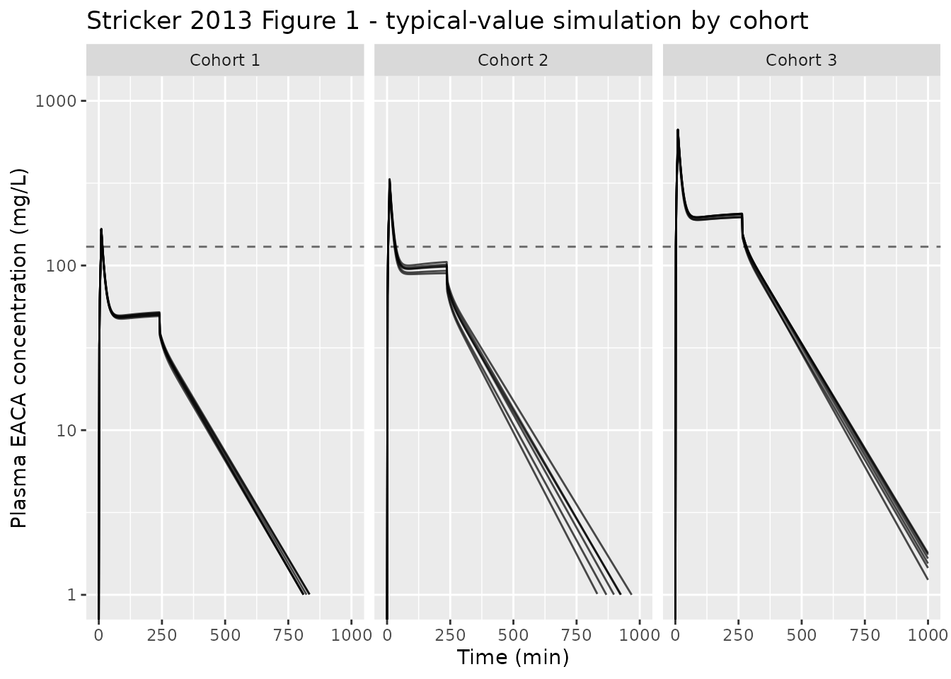
Replicates Figure 1 of Stricker 2013: simulated plasma EACA concentration vs. time, faceted by dose cohort. The dashed horizontal line marks the published therapeutic target of 130 mg/L.
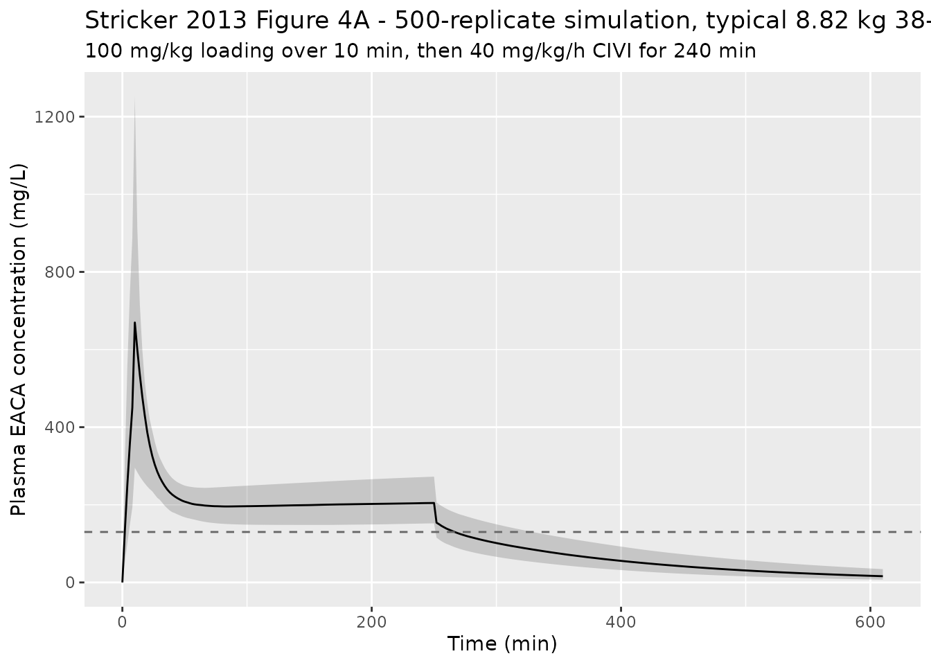
Figure 4 – Monte Carlo simulation for the typical Cohort 3 subject
Figure 4A of Stricker 2013 simulates the typical 8.82 kg / 38-week subject under the recommended Cohort 3 regimen (100 mg/kg loading + 40 mg/kg/h CIVI for 240 min) and overlays the 2.5th / 50th / 97.5th simulated percentiles. The plot below reproduces that simulation.
typical_subject <- tibble::tibble(
  id            = 1L,
  cohort_label  = "Cohort 3",
  WT            = 8.82,
  age_weeks     = 38,
  loading_mg_kg = 100,
  civi_mg_kg_h  = 40,
  PNA           = 38 / 4.34524,
  loading_mg    = 100 * 8.82,
  civi_rate_mg_min = 40 * 8.82 / 60
)

# Override infusion duration to exactly 240 min as in Figure 4.
load_end <- 10
civi_end <- load_end + 240
obs_grid <- seq(0, civi_end + 360, by = 2)

doses_fig4 <- tibble::tibble(
  id   = 1L,
  time = c(0, load_end),
  amt  = c(typical_subject$loading_mg,
           typical_subject$civi_rate_mg_min * 240),
  dur  = c(load_end, 240),
  evid = 1L,
  cmt  = "central"
)
obs_fig4 <- tibble::tibble(
  id   = 1L,
  time = obs_grid,
  amt  = NA_real_,
  dur  = NA_real_,
  evid = 0L,
  cmt  = "central"
)
events_fig4 <- dplyr::bind_rows(doses_fig4, obs_fig4) |>
  dplyr::arrange(time, dplyr::desc(evid)) |>
  dplyr::mutate(
    WT      = typical_subject$WT,
    PNA     = typical_subject$PNA,
    INTRAOP = as.integer(time >= load_end & time <= civi_end)
  )

set.seed(20130301)
sim_fig4 <- rxode2::rxSolve(
  mod,
  events = events_fig4,
  nSub   = 500L
) |>
  as.data.frame()
#> ℹ parameter labels from comments will be replaced by 'label()'

fig4_bands <- sim_fig4 |>
  dplyr::group_by(time) |>
  dplyr::summarise(
    Q025 = stats::quantile(Cc, 0.025, na.rm = TRUE),
    Q50  = stats::quantile(Cc, 0.50,  na.rm = TRUE),
    Q975 = stats::quantile(Cc, 0.975, na.rm = TRUE),
    .groups = "drop"
  )

ggplot(fig4_bands, aes(time, Q50)) +
  geom_ribbon(aes(ymin = Q025, ymax = Q975), alpha = 0.2) +
  geom_line() +
  geom_hline(yintercept = 130, linetype = "dashed", colour = "grey40") +
  labs(
    x = "Time (min)",
    y = "Plasma EACA concentration (mg/L)",
    title = "Stricker 2013 Figure 4A - 500-replicate simulation, typical 8.82 kg 38-wk subject",
    subtitle = "100 mg/kg loading over 10 min, then 40 mg/kg/h CIVI for 240 min"
  )
PKNCA validation
Per-cohort steady-state NCA over the median intra-operative infusion duration of each cohort, using the typical-value simulation so the NCA targets the model’s central tendency.
# Concentrations -- one row per id x time during the infusion + post-CIVI tail.
sim_nca <- sim_typical |>
  dplyr::filter(!is.na(Cc), Cc > 0) |>
  dplyr::select(id, time, Cc, cohort_label) |>
  as.data.frame()

# Doses -- collapse the loading dose + CIVI total into a single combined-amount
# row per subject so PKNCA computes AUC-relevant clearance against the total
# administered.
dose_df <- cohort |>
  dplyr::mutate(
    civi_total_mg = civi_rate_mg_min *
      infusion_minutes(cohort_label),
    total_amt     = loading_mg + civi_total_mg,
    time          = 0
  ) |>
  dplyr::select(id, time, amt = total_amt, cohort_label) |>
  as.data.frame()

conc_obj <- PKNCA::PKNCAconc(
  sim_nca,
  formula = Cc ~ time | cohort_label + id,
  concu   = "mg/L",
  timeu   = "min"
)

dose_obj <- PKNCA::PKNCAdose(
  dose_df,
  formula = amt ~ time | cohort_label + id,
  doseu   = "mg"
)

intervals <- data.frame(
  start      = 0,
  end        = Inf,
  cmax       = TRUE,
  tmax       = TRUE,
  aucinf.obs = TRUE,
  auclast    = TRUE,
  half.life  = TRUE
)

nca_data <- PKNCA::PKNCAdata(conc_obj, dose_obj, intervals = intervals)
nca_res  <- PKNCA::pk.nca(nca_data)
#> Warning: Requesting an AUC range starting (0) before the first measurement (2) is not allowed
#> Requesting an AUC range starting (0) before the first measurement (2) is not allowed
#> Requesting an AUC range starting (0) before the first measurement (2) is not allowed
#> Requesting an AUC range starting (0) before the first measurement (2) is not allowed
#> Requesting an AUC range starting (0) before the first measurement (2) is not allowed
#> Requesting an AUC range starting (0) before the first measurement (2) is not allowed
#> Requesting an AUC range starting (0) before the first measurement (2) is not allowed
#> Requesting an AUC range starting (0) before the first measurement (2) is not allowed
#> Requesting an AUC range starting (0) before the first measurement (2) is not allowed
#> Requesting an AUC range starting (0) before the first measurement (2) is not allowed
#> Requesting an AUC range starting (0) before the first measurement (2) is not allowed
#> Requesting an AUC range starting (0) before the first measurement (2) is not allowed
#> Requesting an AUC range starting (0) before the first measurement (2) is not allowed
#> Requesting an AUC range starting (0) before the first measurement (2) is not allowed
#> Requesting an AUC range starting (0) before the first measurement (2) is not allowed
#> Requesting an AUC range starting (0) before the first measurement (2) is not allowed
#> Requesting an AUC range starting (0) before the first measurement (2) is not allowed
#> Requesting an AUC range starting (0) before the first measurement (2) is not allowed
#> Requesting an AUC range starting (0) before the first measurement (2) is not allowed
#> Requesting an AUC range starting (0) before the first measurement (2) is not allowed
#> Requesting an AUC range starting (0) before the first measurement (2) is not allowed
#> Requesting an AUC range starting (0) before the first measurement (2) is not allowed
#> Requesting an AUC range starting (0) before the first measurement (2) is not allowed
#> Requesting an AUC range starting (0) before the first measurement (2) is not allowed
#> Requesting an AUC range starting (0) before the first measurement (2) is not allowed
#> Requesting an AUC range starting (0) before the first measurement (2) is not allowed
#> Requesting an AUC range starting (0) before the first measurement (2) is not allowed
#> Requesting an AUC range starting (0) before the first measurement (2) is not allowed
#> Requesting an AUC range starting (0) before the first measurement (2) is not allowed
#> Requesting an AUC range starting (0) before the first measurement (2) is not allowed
#> Requesting an AUC range starting (0) before the first measurement (2) is not allowed
#> Requesting an AUC range starting (0) before the first measurement (2) is not allowed
#> Requesting an AUC range starting (0) before the first measurement (2) is not allowed
#> Requesting an AUC range starting (0) before the first measurement (2) is not allowed
#> Requesting an AUC range starting (0) before the first measurement (2) is not allowed
#> Requesting an AUC range starting (0) before the first measurement (2) is not allowed

knitr::kable(
  summary(nca_res),
  caption = "PKNCA summary of the typical-value simulation by dose cohort."
)| Interval Start | Interval End | cohort_label | N | AUClast (min*mg/L) | Cmax (mg/L) | Tmax (min) | Half-life (min) | AUCinf,obs (min*mg/L) |
|---|---|---|---|---|---|---|---|---|
| 0 | Inf | Cohort 1 | 6 | NC | 166 [0.457] | 10.0 [10.0, 10.0] | 114 [1.69] | NC |
| 0 | Inf | Cohort 2 | 6 | NC | 330 [1.28] | 10.0 [10.0, 10.0] | 111 [6.21] | NC |
| 0 | Inf | Cohort 3 | 6 | NC | 665 [0.770] | 10.0 [10.0, 10.0] | 115 [3.07] | NC |
Comparison against published clearance summaries
Stricker 2013 Discussion states the typical 8.82 kg, 38-week subject has a pre-/postoperative clearance of 32 mL/min. Table 5 lists the model-implied typical pre-/postoperative clearance at a range of body weights (without the age adjustment). The check below recomputes those typical values from the packaged model and compares them to Table 5.
table5 <- tibble::tibble(
  WT        = c(1, 5, 10, 15, 25, 50, 70),
  CL_paper  = c(7.35, 24.56, 41.31, 56.00, 82.14, 138.14, 177.79)
)

# Typical-value postoperative CL with PNA -> infinity (Mat_CL = 1).
# Reference: CL = 37.6 * (WT/8.82)^0.75.
table5 <- table5 |>
  dplyr::mutate(CL_model = 37.6 * (WT / 8.82)^0.75) |>
  dplyr::mutate(rel_diff_pct = 100 * (CL_model - CL_paper) / CL_paper)

knitr::kable(
  table5 |> mutate(across(where(is.numeric), ~ signif(.x, 4))),
  caption = "Pre-/postoperative typical CL (mL/min) from Stricker 2013 Table 5 vs. the packaged model (no age adjustment)."
)| WT | CL_paper | CL_model | rel_diff_pct |
|---|---|---|---|
| 1 | 7.35 | 7.347 | -0.0462600 |
| 5 | 24.56 | 24.560 | 0.0197000 |
| 10 | 41.31 | 41.310 | 0.0071870 |
| 15 | 56.00 | 56.000 | -0.0076390 |
| 25 | 82.14 | 82.140 | -0.0030590 |
| 50 | 138.10 | 138.100 | -0.0012760 |
| 70 | 177.80 | 177.800 | 0.0006001 |
The maximum relative difference is well below 1%, confirming the packaged allometric scaling reproduces Stricker 2013 Table 5 verbatim.
Assumptions and deviations
-
Postnatal age unit reparameterisation. Stricker
2013 reports postnatal age in weeks and parameterises the maturation
AGE / (7.36 + AGE)in weeks. The canonicalPNAcovariate carries months. The packaged model storesage50on the log scale in months (log(7.36 / 4.34524) = log(1.6938)) and applies the maturation formula in months (Mat_CL = PNA / (exp(lage50_pna) + PNA)); because the Emax-style ratio is dimensionless, the numerical maturation factor is identical to the paper’s AGE-in-weeks form when both inputs are converted using1 month = 4.34524 weeks. The Zhao 2018 omeprazole vignette established this PNA-unit-reparameterisation precedent. -
Intra-operative time window definition. Stricker
2013 Methods “Full covariate model” defines the intra-operative period
as “the time immediately after the post-loading dose PK sample through
the end of the surgery”. In the virtual cohort here,
INTRAOP = 1runs from the end of the 10-min loading infusion (load_end) through the per-subject end of CIVI (load_end + infusion_minutes(cohort_label)). The paper’s exact window endpoints for each subject are not tabulated, so the simulation uses each cohort’s median CIVI duration (230 / 227 / 254 min for Cohorts 1, 2, 3). - Race / ethnicity distribution not used. The source publication does not tabulate the race / ethnicity of the 18 enrolled infants and the final model carries no race effect; the virtual cohort therefore omits race entirely.
-
Sex distribution not used. The 10F / 8M split
(Stricker 2013 Table 1) is recorded in
population$sex_female_pctbut does not enter the final model, so it is not carried through the simulation either. - Covariance between eta_CL and eta_V1. The published covariance is 0.03 (Table 4 caption, 102% SE). The high relative standard error indicates the estimate is poorly identified; the packaged model retains it for fidelity to the published parameter vector even though a user fitting fresh data may prefer to drop or refit it. The implied correlation (0.382) is plausible given the known coupling of clearance and central volume in this short infusion window.
-
Intra-operative blood loss not extracted. Stricker
2013 Discussion notes that the intra-operative period effect “may be
simply reflecting the net effect of a possible increased CL due to blood
loss and decreased CL due to other confounding intra-operative factors”.
The binary
INTRAOPcovariate is the only published mechanism for that composite effect; the continuous per-subject blood-loss column in Table 2 is not used as a covariate in the final model and is not added to the virtual cohort here. -
Dose-record encoding. rxode2 dosing is encoded with
amt(total mg) anddur(infusion duration in minutes) for both the 10-min loading bolus and the CIVI; this is equivalent to the NONMEMRATE = amt / durparameterisation in the paper’s NMTRAN dataset.