Spatial PK and imipenem PK/PD in airway mucus (Guo 2025)
Source:vignettes/articles/Guo_2025_mucus_spatial_pkpd.Rmd
Guo_2025_mucus_spatial_pkpd.RmdModel and source
Guo 2025 contributes two models, both deterministic simulation frameworks:
Guo_2025_mucus_spatial_pk– the generic spatial PK framework for a hypothetical intravenously dosed drug diffusing across cystic fibrosis (CF) airway mucus.Guo_2025_imipenem_mucus– the imipenem case study, which couples the same mucus diffusion layer to a two-compartment imipenem plasma model and a two-subpopulation Pseudomonas aeruginosa kill model at every grid node.Citation: Guo Y, Yin J, Yonucu S, Knibbe CAJ, Guo T, van Hasselt JGC. Spatial Pharmacokinetic and Pharmacodynamic Modeling in Airway Mucus. Clin Pharmacokinet. 2025;64(12):1869-1883. doi:10.1007/s40262-025-01575-4. Equations 1-5 and Table 1 of the article, Equation S1 and Table S1 of the supplement; plasma volume, infusion duration and molecular weight from the authors’ deposited code (https://github.com/vanhasseltlab/spatialPK).
Description (framework): Mechanistic spatial PK (method-of-lines discretised PDE). Diffusion of a hypothetical intravenously dosed drug across a 500 um layer of cystic fibrosis airway mucus (Guo 2025). A one-compartment plasma model sets the free concentration at the blood-mucus interface (instantaneous transfer, partition 1, no protein binding); within mucus the free drug diffuses by Fick’s second law with a Stokes-Einstein diffusion coefficient computed from the molecule/particle radius and a mucin-dependent micro-viscosity, binds reversibly to immobile mucins (kon, koff) and is removed with muco-ciliary clearance (free and bound alike); the air-mucus interface is a zero-flux face. The layer is discretised on the authors’ 25 um grid (21 nodes; 19 free and 20 bound drug states). Defaults are the paper’s Table 1 small molecule (r = 1 nm, D = 78.6 um^2/s, t1/2 3 h); the radius, half-life, mucin, binding and muco-ciliary knobs reproduce the Figure 3-5 sweeps. No inter-individual or residual variability (simulation framework).
Description (imipenem): Mechanistic spatial PK/PD (method-of-lines discretised PDE). Imipenem killing of Pseudomonas aeruginosa inside a 500 um layer of cystic fibrosis airway mucus (Guo 2025 case study). Plasma PK is the two-compartment imipenem model of van Hasselt 2016 (CL 11.52 L/h, V1 9.37 L, V2 6.41 L, Q 13.68 L/h); the free concentration at the blood-mucus interface is the plasma concentration times the ELF penetration coefficient 0.444. Within mucus imipenem diffuses (Fick’s second law, Stokes-Einstein D for r = 1 nm, about 78.6 um^2/s) and binds reversibly to immobile mucins; muco-ciliary clearance is set to zero. Immobile bacteria at every grid node follow a two-subpopulation (susceptible S, resistant R) logistic-growth model with linear concentration-driven kill and drug-independent S-to-R transfer. The layer is discretised on the authors’ 25 um grid (21 nodes; 19 free drug, 20 bound drug, 20 S and 20 R states). The baseline inoculum is homogeneous at 10^5.67 CFU/mL; per-node log10 offsets (dlog10b0_slab
) give gradient baselines. Deterministic: no inter-individual or residual variability. Article: https://doi.org/10.1007/s40262-025-01575-4 (open access, PMC12715044)
Authors’ code: https://github.com/vanhasseltlab/spatialPK
Population
No patients were studied. The paper simulates hypothetical drugs and a typical adult, with physiological mucus parameters taken from CF sputum and mucus-plug literature (Table 1 and Table S1): a 500 um mucus layer, total mucin 2e-5 mol/L, a mucin-dependent micro-viscosity (Equation S1) and muco-ciliary clearance 0.036 1/h. Hypothetical drugs vary in molecule/particle radius (1, 5, 20, 50 nm), plasma half-life, mucin binding affinity, mucin concentration and muco-ciliary clearance. The imipenem case study uses the pooled imipenem plasma model of van Hasselt 2016 and in vitro P. aeruginosa time-kill parameters (Table S2).
readModelDb("Guo_2025_mucus_spatial_pk")()$population$notes
#> [1] "No patients were studied. Hypothetical drugs spanning molecule/particle radius 1, 5, 20 and 50 nm, plasma half-life 3-24 h (small) or 1-4 weeks (large), mucin association constant 10-10000 1/M, total mucin 1e-6 to 5e-5 mol/L and muco-ciliary clearance 0-0.36 1/h were simulated against CF physiological mucus parameters (Table 1, Table S1)."
readModelDb("Guo_2025_imipenem_mucus")()$population$notes
#> [1] "No patients were studied. A typical-value plasma PK model (van Hasselt 2016) drives the mucus boundary condition; bacterial PD parameters come from in vitro P. aeruginosa time-kill data (Guo 2024 bioRxiv). Three baseline bacterial spatial organisations (homogeneous, increasing and decreasing gradient) were simulated (Fig. S1, Table S3)."
Model structure
The mucus layer obeys Equations 4-5 of the paper:
- free drug
A(x, t):dA/dt = D d2A/dx2 - kon (M - A') A + koff A' - ke,m A - mucin-bound drug
A'(x, t):dA'/dt = kon (M - A') A - koff A' - ke,m A'
with A(0, t) equal to the plasma concentration (the
imipenem model multiplies it by the ELF penetration coefficient 0.444),
A = A' = 0 at t = 0, and a zero-flux air-mucus
interface. The diffusion coefficient comes from the modified
Stokes-Einstein equation (Equation 2),
D = kB T / (6 c pi mu r), with c = 2/3 for r
<= 1 nm (else 1) and the micro-viscosity
mu = 128.87 M + 0.00176 (Equation S1).
rxode2 solves ODEs, so the PDE is written by the method of lines on
the authors’ own spatial grid: 25 um steps over 500 um, i.e. 21 nodes at
x = (n - 1) * 25 um. Node 1 is the blood-mucus interface,
whose free concentration is the boundary value Cmucus_bc
(an algebraic output, not a state). Nodes 2-20 carry the free-drug
states mucus_free_slab2 … mucus_free_slab20,
nodes 1-20 carry the bound-drug states mucus_bound_slab1 …
mucus_bound_slab20, and node 21 is a copy of node 20, which
is how the authors’ finite-difference code imposes the reflective
air-mucus face. The authors integrated in time with an explicit 0.5 s
step; rxode2 integrates the same spatial discretisation with an adaptive
solver. The reproduction of every published AUC below (all within 1%) is
the evidence that this grid and the time integration are adequate.
Convenience outputs: Cmucus_free_mean and
Cmucus_bound_mean (mean over the 21 nodes) and
Cmucus_free_cv (the paper’s spatial-heterogeneity metric,
coefficient of variation of the free concentration across nodes, in
percent). The paper’s exposure metric AUCf (“double integral of free
drug concentration in mucus over time and distance”, reported in mg*h/L)
is the time integral of Cmucus_free_mean; this is how the
authors’ code computes it.
In the imipenem model each node 1-20 also carries susceptible
(bact_susceptible_slab<n>) and resistant
(bact_resistant_slab<n>) bacteria in CFU/mL
(Equations S2-S3), killed by the local free imipenem concentration;
bact_total_mean is the node-averaged total.
Source trace
| Equation / parameter | Value | Source location |
|---|---|---|
| Fick’s second law, Eq. 1 / mucus PDEs | n/a | Equations 1, 4, 5 |
Stokes-Einstein D, c = 2/3 for r <= 1
nm |
n/a | Equation 2 and text below it |
Micro-viscosity mu = 128.87 M + 0.00176
|
visc_slope, visc_int
|
Equation S1 |
kboltz |
1.380649e-23 N*m/K | Table S1 |
temp_k |
310 K | Table S1 |
r_hyd |
1 nm (framework default) | Table 1 title; Table S1 |
thick_mucus |
500 um | Table 1, Table S2 |
mucin |
2e-5 mol/L | Table 1, Table S2 |
kon, koff
|
100 1/(M*s), 0.1 1/s | Table 1, Table S2 |
kel_mcc (framework) |
0.036 1/h | Table 1 (printed 0.04), Fig. 4 caption (0.036), Table S1 (1e-5 1/s) |
kel_mcc (imipenem) |
0 | Table S2 |
| Plasma one-compartment model | n/a | Equation 3 |
lcl, lvc (framework) |
3.465 L/h, 15 L | authors’ code; reproduces the 3 h half-life of Fig. 4 |
mw |
500 g/mol | authors’ code (pde()) |
| Spatial grid | 25 um, 21 nodes | Methods, Algorithm and Software |
Imipenem lcl, lvc, lvp,
lq
|
11.52 L/h, 9.37 L, 6.41 L, 13.68 L/h | Table S2 (L/min x 60) |
relf |
0.444 | Table S2 P_ELF
|
kgs, kgr, ksr
|
1.67e-4, 0, 9.86e-6 1/s | Table S2 |
slope_s, slope_r
|
2.38e-4, 3.78e-5 L/(mg*s) | Table S2 |
log10b0, log10bmax
|
5.67, 9.52 log10 CFU/mL | Table S2 |
| Bacterial PD ODEs | n/a | Equations S2-S3 |
Simulation helpers
mod_pk <- readModelDb("Guo_2025_mucus_spatial_pk")
mod_pd <- readModelDb("Guo_2025_imipenem_mucus")

obs_grid <- seq(0, 72, by = 1 / 60)

# IV regimens; every dose is an infusion into the plasma compartment
regimen <- function(amt, ii, dur, end = 72) {
  et(amt = amt, dur = dur, ii = ii, addl = end / ii - 1, cmt = "central") |>
    et(seq(0, end, by = 1 / 60))
}

solve_scenario <- function(mod, ev, params = NULL, label) {
  s <- rxSolve(mod, ev, params = params, returnType = "data.frame")
  s$scenario <- label
  s$id <- 1L
  s
}

# Free concentration at each of the 21 grid nodes (node 21 = node 20)
free_long <- function(s) {
  free <- cbind(
    s$Cmucus_bc,
    as.matrix(s[, paste0("mucus_free_slab", 2:20)]),
    s$mucus_free_slab20
  )
  data.frame(
    time = rep(s$time, 21),
    distance = rep((0:20) * 25, each = nrow(s)),
    conc = as.vector(free),
    plasma = rep(s$Cc, 21)
  )
}
Diffusion coefficients
The paper reports D of about 78.6 um^2/s for r = 1 nm,
10.5 um^2/s for r = 5 nm, and 1.0-2.6 um^2/s for r = 20-50 nm at 2e-5
mol/L mucin.
d_tab <- bind_rows(lapply(c(1, 5, 20, 50), function(r) {
  s <- rxSolve(mod_pk, et(0), params = c(r_hyd = r), returnType = "data.frame")
  data.frame(`Radius (nm)` = r, `D (um^2/s)` = signif(s$diff_coef[1], 3), check.names = FALSE)
}))
knitr::kable(d_tab)| Radius (nm) | D (um^2/s) |
|---|---|
| 1 | 78.50 |
| 5 | 10.50 |
| 20 | 2.62 |
| 50 | 1.05 |
stopifnot(
  abs(d_tab[[2]][1] - 78.6) < 0.2,
  abs(d_tab[[2]][2] - 10.5) < 0.1,
  round(d_tab[[2]][3], 1) == 2.6, round(d_tab[[2]][4], 1) == 1.0
)
Using the rounded coefficients printed in Equation S1, r = 1 nm gives
78.5 um^2/s rather than the printed 78.6. The authors’ code carries
unrounded coefficients (0.001 * (1.756757 + 1.288649e5 M)),
which give 78.6 exactly; the 0.1% difference has no visible effect on
any output below.
Figure 2: small molecule, 100 mg every 8 h
s_fig2 <- solve_scenario(mod_pk, regimen(100, 8, 0.5, end = 24), label = "fig2")
f2 <- free_long(s_fig2)

ggplot(s_fig2, aes(time, Cc)) +
  geom_line() +
  labs(x = "Time (h)", y = "Plasma concentration (mg/L)",
       title = "Replicates Figure 2A of Guo 2025")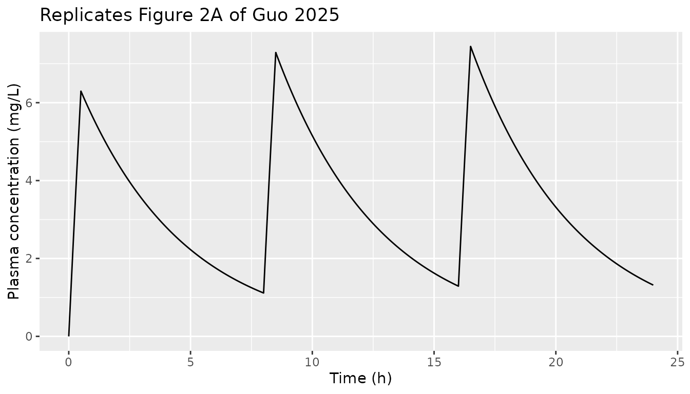
f2_plot <- f2 |> filter(abs(time * 12 - round(time * 12)) < 1e-6)
ggplot(f2_plot, aes(time, distance, fill = conc)) +
  geom_tile() +
  scale_fill_distiller("Free conc.\n(mg/L)", palette = 4, direction = 1) +
  labs(x = "Time (h)", y = "Distance (um)", title = "Replicates Figure 2B of Guo 2025")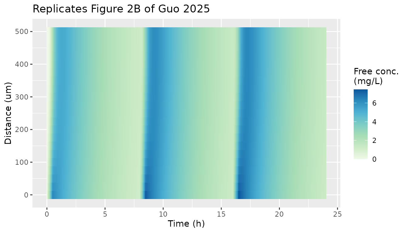
ggplot(f2_plot |> filter(plasma > 0), aes(time, distance, fill = conc / plasma)) +
  geom_tile() +
  scale_fill_distiller("Mucus:plasma", palette = 4, direction = 1) +
  labs(x = "Time (h)", y = "Distance (um)", title = "Replicates Figure 2C of Guo 2025")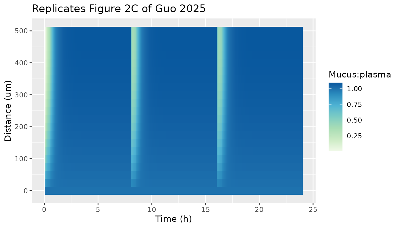
ggplot(s_fig2 |> filter(time > 0), aes(time, Cmucus_free_cv)) +
  geom_line() +
  labs(x = "Time (h)", y = "Spatial CV of free conc. (%)",
       title = "Replicates Figure 2D of Guo 2025")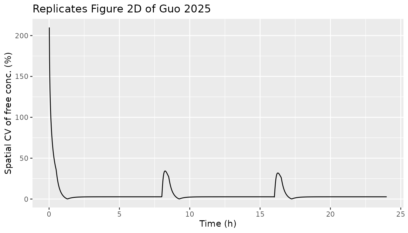
# The paper: the mucus:plasma ratio reaches 1 within 2 h of every dose and the
# spatial CV drops below 3% about 1 h after every administration.
ratio_2h <- f2 |> filter(abs(time - 18) < 1e-6) |> summarise(r = min(conc / plasma))
cv_1h <- s_fig2 |> filter(time > 17.5, time < 17.6) |> pull(Cmucus_free_cv)
ratio_2h
#>   r
#> 1 1
range(cv_1h)
#> [1] 1.461454 1.674233
stopifnot(ratio_2h$r > 0.95, all(cv_1h < 5))
Figure 3 and Figure 4A: drug- and system-specific factors
All scenarios are 100 mg every 8 h (0.5 h infusion) for 72 h; each
factor is varied with the others at their reference values
(t1/2 = 3 h, r = 1 nm, Ka = 1000 1/M,
M = 2e-5 mol/L, ke,m = 0.036 1/h). The binding
affinity Ka = kon / koff is varied through kon
at the fixed koff = 0.1 1/s.
q8 <- regimen(100, 8, 0.5)
sweep_def <- bind_rows(
  data.frame(factor = "Radius", scenario = paste0("r = ", c(1, 5, 20, 50), " nm"),
             par = "r_hyd", value = c(1, 5, 20, 50)),
  data.frame(factor = "Half-life", scenario = paste0("t1/2 = ", c(3, 6, 12, 24), " h"),
             par = "lcl", value = log(c(0.05775, 0.0289, 0.01444, 0.00722) * 60)),
  data.frame(factor = "Binding", scenario = paste0("Ka = ", c(10, 100, 1000, 10000), " 1/M"),
             par = "kon", value = c(10, 100, 1000, 10000) * 0.1),
  data.frame(factor = "Mucin", scenario = paste0("M = ", c("1e-6", "5e-6", "1e-5", "5e-5"), " mol/L"),
             par = "mucin", value = c(1e-6, 5e-6, 1e-5, 5e-5)),
  data.frame(factor = "Muco-ciliary", scenario = paste0("ke,m = ", c(0, 0.0036, 0.036, 0.36), " 1/h"),
             par = "kel_mcc", value = c(0, 0.0036, 0.036, 0.36))
)
sweep_sims <- bind_rows(lapply(seq_len(nrow(sweep_def)), function(i) {
  solve_scenario(mod_pk, q8, params = setNames(sweep_def$value[i], sweep_def$par[i]),
                 label = sweep_def$scenario[i])
}))
radius_long <- bind_rows(lapply(paste0("r = ", c(1, 5, 20, 50), " nm"), function(sc) {
  free_long(sweep_sims |> filter(scenario == sc)) |> mutate(scenario = sc)
})) |>
  filter(abs(time * 6 - round(time * 6)) < 1e-6) |>
  mutate(scenario = factor(scenario, levels = paste0("r = ", c(1, 5, 20, 50), " nm")))
ggplot(radius_long, aes(time, distance, fill = conc)) +
  geom_tile() +
  facet_wrap(~scenario, ncol = 1) +
  scale_fill_distiller("Free conc.\n(mg/L)", palette = 4, direction = 1) +
  labs(x = "Time (h)", y = "Distance (um)", title = "Replicates Figure 3A of Guo 2025")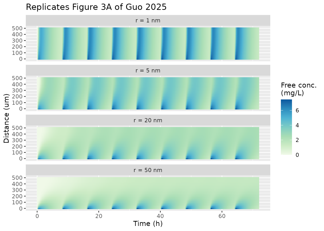
AUCf is computed with PKNCA on the node-averaged free concentration
(Cmucus_free_mean) over 0-72 h with linear trapezoids.
nca_auc72 <- function(sims) {
  # Keep only the columns PKNCA needs; the full simulation is ~100 columns wide.
  conc_data <- sims |>
    select(scenario, id, time, Cmucus_free_mean) |>
    filter(!is.na(Cmucus_free_mean))
  conc <- PKNCAconc(conc_data, Cmucus_free_mean ~ time | scenario / id)
  PKNCAdata(conc, intervals = data.frame(start = 0, end = 72, auclast = TRUE),
            options = list(auc.method = "linear")) |>
    pk.nca() |>
    suppressMessages()
}
sweep_nca <- nca_auc72(sweep_sims)

# Published AUCf (mg*h/L): Results text for radius and half-life; for binding,
# mucin and muco-ciliary clearance the paper reports only the 231-254 range.
ref_sweep <- data.frame(
  scenario = c(paste0("r = ", c(1, 5, 20, 50), " nm"), paste0("t1/2 = ", c(3, 6, 12, 24), " h")),
  auclast = c(251, 232, 183, 133, 251, 474, 831, 1276)
)
cmp_sweep <- ncaComparisonTable(
  sweep_nca |> as.data.frame() |> filter(scenario %in% ref_sweep$scenario),
  ref_sweep, by = "scenario", units = c(auclast = "mg*h/L")
)
knitr::kable(cmp_sweep, caption = "AUCf over 72 h: published (Figures 3B and 4A) vs simulated.")| NCA parameter | scenario | Reference | Simulated | % diff |
|---|---|---|---|---|
| AUClast (mg*h/L) | r = 1 nm | 251 | 251 | +0.0% |
| AUClast (mg*h/L) | r = 5 nm | 232 | 232 | -0.0% |
| AUClast (mg*h/L) | r = 20 nm | 183 | 183 | -0.2% |
| AUClast (mg*h/L) | r = 50 nm | 133 | 133 | -0.0% |
| AUClast (mg*h/L) | t1/2 = 3 h | 251 | 251 | +0.0% |
| AUClast (mg*h/L) | t1/2 = 6 h | 474 | 474 | -0.0% |
| AUClast (mg*h/L) | t1/2 = 12 h | 831 | 831 | -0.0% |
| AUClast (mg*h/L) | t1/2 = 24 h | 1280 | 1280 | -0.1% |
auc_check <- function(nca, ref) {
  sim <- as.data.frame(nca) |> filter(PPTESTCD == "auclast") |> select(scenario, sim = PPORRES)
  inner_join(ref, sim, by = "scenario") |> mutate(pct = 100 * (sim - auclast) / auclast)
}
# Deterministic model: the only difference from the paper is numerical.
stopifnot(all(abs(auc_check(sweep_nca, ref_sweep)$pct) < 1))

other <- as.data.frame(sweep_nca) |>
  filter(PPTESTCD == "auclast", !scenario %in% ref_sweep$scenario)
knitr::kable(other |> select(Scenario = scenario, `AUCf (mg*h/L)` = PPORRES) |>
               mutate(`AUCf (mg*h/L)` = round(`AUCf (mg*h/L)`, 1)),
caption = "Binding, mucin and muco-ciliary sweeps; the paper reports 231-254 mg*h/L.")| Scenario | AUCf (mg*h/L) |
|---|---|
| Ka = 10 1/M | 251.1 |
| Ka = 100 1/M | 251.1 |
| Ka = 1000 1/M | 251.0 |
| Ka = 10000 1/M | 250.6 |
| ke,m = 0 1/h | 253.6 |
| ke,m = 0.0036 1/h | 253.3 |
| ke,m = 0.036 1/h | 251.0 |
| ke,m = 0.36 1/h | 230.5 |
| M = 1e-5 mol/L | 251.9 |
| M = 1e-6 mol/L | 252.7 |
| M = 5e-5 mol/L | 248.2 |
| M = 5e-6 mol/L | 252.4 |
Peak spatial CV after the last administration (Figure 3C; paper: 29.9%, 48.6%, 47.5% and 62.9% for 1, 5, 20 and 50 nm):
peak_cv <- sweep_sims |>
  filter(grepl("^r = ", scenario), time > 64, time <= 72) |>
  group_by(scenario) |>
  summarise(simulated = max(Cmucus_free_cv, na.rm = TRUE), .groups = "drop") |>
  mutate(published = c("r = 1 nm" = 29.9, "r = 20 nm" = 47.5, "r = 5 nm" = 48.6,
                       "r = 50 nm" = 62.9)[scenario]) |>
  arrange(published)
knitr::kable(peak_cv |> rename(Scenario = scenario, `Simulated peak CV (%)` = simulated,
`Published peak CV (%)` = published), digits = 1)| Scenario | Simulated peak CV (%) | Published peak CV (%) |
|---|---|---|
| r = 1 nm | 31.5 | 29.9 |
| r = 20 nm | 47.4 | 47.5 |
| r = 5 nm | 48.4 | 48.6 |
| r = 50 nm | 62.8 | 62.9 |
The peak CV is the extreme of a fast transient at the start of each infusion, so it is sensitive to time resolution: the authors’ explicit scheme updates the boundary value once a minute, while rxode2 follows the plasma profile continuously. The 1 nm value is 1.6 points higher here; the larger molecules, whose transients are slower, agree within 0.2 points.
Figure 5: dosing schedule at a fixed 300 mg/day
sched <- list(
  "q8h" = regimen(100, 8, 0.5),
  "q24h" = regimen(300, 24, 0.5),
  "continuous" = et(amt = 900, dur = 72, cmt = "central") |> et(obs_grid)
)
sched_sims <- bind_rows(lapply(c(1, 50), function(r) {
  bind_rows(lapply(names(sched), function(nm) {
    solve_scenario(mod_pk, sched[[nm]], params = c(r_hyd = r),
                   label = paste0("r = ", r, " nm, ", nm))
  }))
}))
sched_nca <- nca_auc72(sched_sims)
ref_sched <- data.frame(
  scenario = paste0("r = ", rep(c(1, 50), each = 3), " nm, ", rep(names(sched), 2)),
  auclast = c(251, 257, 241, 133, 145, 125)
)
cmp_sched <- ncaComparisonTable(sched_nca, ref_sched, by = "scenario",
                                units = c(auclast = "mg*h/L"))
knitr::kable(cmp_sched, caption = "AUCf over 72 h by dosing schedule: published (Figure 5B) vs simulated.")| NCA parameter | scenario | Reference | Simulated | % diff |
|---|---|---|---|---|
| AUClast (mg*h/L) | r = 1 nm, q8h | 251 | 251 | +0.0% |
| AUClast (mg*h/L) | r = 1 nm, q24h | 257 | 257 | -0.1% |
| AUClast (mg*h/L) | r = 1 nm, continuous | 241 | 241 | -0.1% |
| AUClast (mg*h/L) | r = 50 nm, q8h | 133 | 133 | -0.0% |
| AUClast (mg*h/L) | r = 50 nm, q24h | 145 | 145 | -0.3% |
| AUClast (mg*h/L) | r = 50 nm, continuous | 125 | 125 | +0.2% |
Imipenem spatial PK/PD (Figure 6, Table S3)
Six regimens (250, 500 or 1000 mg every 8 h, as 0.5 h infusions or as a continuous infusion of the same daily amount) are combined with three baseline bacterial organisations. The gradient baselines follow the authors’ code: 21 log10 densities drawn from a Poisson distribution with mean 5.58 and sorted increasing (more bacteria at the air-mucus face) or decreasing (more at the blood-mucus face). R’s Poisson generator is deterministic for a given seed, so the draw below is the authors’ own. Time to eradication (TTE) is the first time the total density is below 1 CFU/mL at every node.
set.seed(2022)
lognum <- rpois(21, 5.58)
baselines <- list(
  homogeneous = rep(5.67, 20),
  increasing = sort(lognum)[1:20],
  decreasing = sort(lognum, decreasing = TRUE)[1:20]
)
offsets <- function(b, b0 = 5.67) setNames(b - b0, paste0("dlog10b0_slab", 1:20))

imi_regimens <- list(
  "intermittent 250 mg" = regimen(250, 8, 0.5), "intermittent 500 mg" = regimen(500, 8, 0.5),
  "intermittent 1000 mg" = regimen(1000, 8, 0.5), "continuous 250 mg" = regimen(250, 8, 8),
  "continuous 500 mg" = regimen(500, 8, 8), "continuous 1000 mg" = regimen(1000, 8, 8)
)

tte <- function(s) {
  tot <- as.matrix(s[, paste0("bact_susceptible_slab", 1:20)]) +
    as.matrix(s[, paste0("bact_resistant_slab", 1:20)])
  i <- which(apply(tot, 1, max) < 1 & s$time > 0)
  if (length(i) == 0) NA_real_ else s$time[i[1]]
}

imi_sims <- list()
tte_tab <- expand.grid(regimen = names(imi_regimens), baseline = names(baselines),
                       stringsAsFactors = FALSE)
tte_tab$tte_model <- NA_real_
tte_tab$tte_b0_558 <- NA_real_
for (k in seq_len(nrow(tte_tab))) {
  ev <- imi_regimens[[tte_tab$regimen[k]]]
  b <- baselines[[tte_tab$baseline[k]]]
  s <- rxSolve(mod_pd, ev, params = offsets(b), returnType = "data.frame")
  imi_sims[[paste(tte_tab$regimen[k], tte_tab$baseline[k])]] <- s
  tte_tab$tte_model[k] <- tte(s)
  if (tte_tab$baseline[k] == "homogeneous") {
    s558 <- rxSolve(mod_pd, ev, params = c(log10b0 = 5.58, offsets(rep(5.58, 20), 5.58)),
                    returnType = "data.frame")
    tte_tab$tte_b0_558[k] <- tte(s558)
  }
}
tte_tab$published <- c(
  57.2, 25.3, 10.1, NA, 34.5, 17.2, # homogeneous
  NA, 41.7, 18.4, NA, 51.4, 25.6, # increasing gradient
  NA, 40.7, 17.4, NA, 50.2, 24.8 # decreasing gradient
)
knitr::kable(
  tte_tab |>
    mutate(across(c(tte_model, tte_b0_558), ~ round(.x, 1))) |>
    rename(Regimen = regimen, Baseline = baseline,
           `TTE, model default B0 5.67 (h)` = tte_model,
           `TTE, B0 5.58 (h)` = tte_b0_558,
           `Table S3 (h)` = published),
  caption = paste("Time to complete eradication within 72 h (NA = not achieved).",
                  "The B0 5.58 column applies to the homogeneous baseline only.")
)| Regimen | Baseline | TTE, model default B0 5.67 (h) | TTE, B0 5.58 (h) | Table S3 (h) |
|---|---|---|---|---|
| intermittent 250 mg | homogeneous | 57.8 | 57.4 | 57.2 |
| intermittent 500 mg | homogeneous | 25.6 | 25.4 | 25.3 |
| intermittent 1000 mg | homogeneous | 10.4 | 10.2 | 10.1 |
| continuous 250 mg | homogeneous | NA | NA | NA |
| continuous 500 mg | homogeneous | 35.2 | 34.6 | 34.5 |
| continuous 1000 mg | homogeneous | 17.6 | 17.2 | 17.2 |
| intermittent 250 mg | increasing | NA | NA | NA |
| intermittent 500 mg | increasing | 41.8 | NA | 41.7 |
| intermittent 1000 mg | increasing | 18.5 | NA | 18.4 |
| continuous 250 mg | increasing | NA | NA | NA |
| continuous 500 mg | increasing | 51.5 | NA | 51.4 |
| continuous 1000 mg | increasing | 25.7 | NA | 25.6 |
| intermittent 250 mg | decreasing | NA | NA | NA |
| intermittent 500 mg | decreasing | 40.7 | NA | 40.7 |
| intermittent 1000 mg | decreasing | 17.5 | NA | 17.4 |
| continuous 250 mg | decreasing | NA | NA | NA |
| continuous 500 mg | decreasing | 50.3 | NA | 50.2 |
| continuous 1000 mg | decreasing | 24.8 | NA | 24.8 |
gr <- tte_tab |> filter(baseline != "homogeneous")
hom <- tte_tab |> filter(baseline == "homogeneous")
stopifnot(
  identical(is.na(tte_tab$tte_model), is.na(tte_tab$published)),
  all(abs(gr$tte_model - gr$published) < 0.5, na.rm = TRUE),
  all(abs(hom$tte_b0_558 - hom$published) < 0.5, na.rm = TRUE),
  all(abs(hom$tte_model / hom$published - 1) < 0.05, na.rm = TRUE)
)
bact_long <- function(s, label) {
  tot <- cbind(
    as.matrix(s[, paste0("bact_susceptible_slab", 1:20)]) +
      as.matrix(s[, paste0("bact_resistant_slab", 1:20)])
  )
  tot <- cbind(tot, tot[, 20])
  data.frame(time = rep(s$time, 21), distance = rep((0:20) * 25, each = nrow(s)),
             log_cfu = pmax(log10(as.vector(tot)), 0), panel = label)
}
fig6 <- bind_rows(
  bact_long(imi_sims[["intermittent 500 mg homogeneous"]], "500 mg q8h, homogeneous"),
  bact_long(imi_sims[["intermittent 500 mg increasing"]], "500 mg q8h, increasing gradient"),
  bact_long(imi_sims[["continuous 500 mg homogeneous"]], "500 mg/8 h continuous, homogeneous")
) |> filter(abs(time * 4 - round(time * 4)) < 1e-6)
ggplot(fig6, aes(time, distance, fill = log_cfu)) +
  geom_tile() +
  facet_wrap(~panel, ncol = 1) +
  scale_fill_distiller("Bacteria\n(log10 CFU/mL)", palette = 7, direction = 1) +
  labs(x = "Time (h)", y = "Distance (um)", title = "Replicates Figure 6B-C of Guo 2025")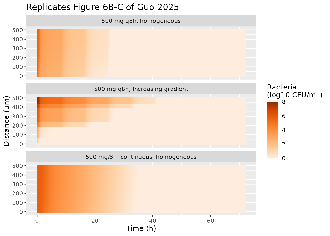
Assumptions and deviations
-
Values taken from the authors’ code. The article
does not print the plasma volume of the hypothetical drug, the infusion
duration, or the molecular weight that converts bound drug to mol/L in
the binding term. They are taken from the authors’ public repository:
V = 15 LwithCL = 0.05775 L/min(a 3 h half-life; the half-life sweep keepsVand changesCL), 0.5 h infusions, andMW = 500 g/mol. Continuous infusion is the daily amount infused over the whole dosing interval. -
Muco-ciliary clearance. Table 1 prints
ke,m = 0.04 1/h; the Figure 4 caption, Table S1 (1e-5 1/s) and the code use 0.036 1/h, which the framework model carries. Table S2 sets it to 0 for imipenem. -
Diffusion coefficient for imipenem. Table S2 lists
D = 79 um^2/sdirectly; the model derives it from the Stokes-Einstein equation with r = 1 nm, as the authors’ code does, giving 78.5 um^2/s. -
Baseline bacterial density. Table S2 gives
B0 = 5.67 log10 CFU/mL, which is the model default. The authors’ code seeds the homogeneous baseline at 5.58 log10 CFU/mL and reproduces Table S3 to within 0.3 h at that value (column “B0 5.58”); at 5.67 the homogeneous TTEs are 1-3% longer. The gradient baselines are absolute per-node densities and do not depend onB0. -
Gradient baselines. These are a random draw in the
authors’ code. The model accepts any baseline through the 20 per-node
offsets
dlog10b0_slab<n>(log10 CFU/mL relative tolog10b0); the draw at node 21 is discarded because node 21 copies node 20. - Regimen in the authors’ code. The deposited imipenem script doses every 6 h; the article and Table S3 use every 8 h, which this vignette follows and which reproduces Table S3.
-
Large-molecule half-life sweep (Figure 4B). The
script for the 600 mg every 2 weeks large-molecule scenarios is not in
the repository and the article does not print their plasma volume, so
the mg*day/L AUCf values of Figure 4B are not compared here. The model
reproduces them once a volume is supplied through
lvcandlcl. -
Boundary condition and plasma model. Mass transfer
from plasma to mucus is instantaneous with partition coefficient 1
(0.444 for imipenem) and the mucus layer does not deplete plasma
(“infinite source”), as in the paper. Delayed boundary conditions and
other mucus thicknesses (Figures S7-S9) are supplement sensitivity
analyses:
thick_mucuschanges the grid step (dx = L / 20), whereas the authors keptdx = 25 umand changed the node count. - No variability. The paper is a deterministic simulation framework; neither model has inter-individual or residual variability.