Gentamicin re-estimated models in critically ill adults (Duong 2022)
Source:vignettes/articles/Duong_2022_gentamicin.Rmd
Duong_2022_gentamicin.RmdModel and source
Duong et al. externally evaluated four published gentamicin
population PK models for critically ill patients against routine
therapeutic drug monitoring data from two Quebec hospitals. None of them
met the bias and imprecision criteria (population MDPE within +/- 20%,
MADPE <= 30%), so each was re-estimated in NONMEM 7.5 on the combined
Quebec data, keeping its original structure and covariates. This article
covers the four re-estimated models. The original
parameter sets belong to the four source papers and are not packaged
here. Hodiamont 2017 (Ther Drug Monit) is packaged separately as
Hodiamont_2017_gentamicin.
| Model file | Structure re-estimated | Original source |
|---|---|---|
Duong_2022_gentamicin_rea |
1-cmt, sigmoid eGFR on CL, WT on V | Rea 2008, Ther Drug Monit 30:674 |
Duong_2022_gentamicin_bos |
1-cmt, linear CrCl on CL | Bos 2019, Antimicrob Agents Chemother 63:e02328-18 |
Duong_2022_gentamicin_hodiamont2017ijaa |
2-cmt, IBW on CL and V1, albumin on V1 | Hodiamont 2017, Int J Antimicrob Agents 49:204 |
Duong_2022_gentamicin_hodiamont2017tdm |
2-cmt, WT on CL, Q and V1 | Hodiamont 2017, Ther Drug Monit 39:522 |
- Citation: Duong A, Simard C, Williamson D, Marsot A. Model Re-Estimation: An Alternative for Poor Predictive Performance during External Evaluations? Example of Gentamicin in Critically Ill Patients. Pharmaceutics 2022;14(7):1426. doi:10.3390/pharmaceutics14071426. Structural model from Rea RS, Capitano B, Bies R, Bigos KL, Smith R, Lee H. Suboptimal aminoglycoside dosing in critically ill patients. Ther Drug Monit 2008;30(6):674-681. doi:10.1097/FTD.0b013e31818b6b2f.
- Article: https://doi.org/10.3390/pharmaceutics14071426
- Supplement (Tables S1-S7): https://www.mdpi.com/article/10.3390/pharmaceutics14071426/s1
The re-estimated Rea model was the only one with acceptable population bias and imprecision (MDPE 2.14%, MADPE 28.1%; Table 2). The authors chose it as the best performing model and used it for the dosing simulations in Tables S5 to S7.
Population
The data come from 87 adult ICU patients reviewed retrospectively. Thirty-nine were treated at the Hopital du Sacre-Coeur de Montreal (HSCM, 2009-2019), mostly for sepsis. Forty-eight were treated at the Institut universitaire de cardiologie et pneumologie de Quebec (IUCPQ, 2014-2020), mostly for endocarditis. All received at least one gentamicin dose and had at least one serum concentration. The combined cohort (Duong 2022 Table 1) had these characteristics:
- 54 male and 33 female patients (37.9% female).
- Age 59.4 +/- 17.9 years and weight 80.0 +/- 21.5 kg.
- Serum creatinine 96.9 +/- 66.0 umol/L, Cockcroft-Gault CrCl 92.2 +/- 48.9 mL/min and MDRD eGFR 80.9 +/- 31.9 mL/min.
- Albumin 29.0 +/- 5.6 g/L, recorded at IUCPQ only.
- Total daily dose 2.4 +/- 1.1 mg/kg.
Height was not among the extracted variables.
The same information is available programmatically through each
model’s population metadata,
e.g. readModelDb("Duong_2022_gentamicin_rea")()$population.
Source trace
Every ini() value carries an in-file comment pointing to
its source. The table collects them. “S1”, “S2”, “S3” and “S4” are
supplementary Tables S1-S4.
| Model | Parameter | Value | Source location |
|---|---|---|---|
| rea |
lclmax (thetaCL,a) |
log(9.31 L/h) | Table S2 |
| rea |
lcrcl50 (thetaCL,b) |
log(129 mL/min) | Table S2 |
| rea | lhill |
fixed(log(1.2)) | Table S2 equation; unchanged from Table S1 |
| rea | lvc |
log(21.7 L) | Table S2 |
| rea | e_wt_vc |
fixed(1) | Table S2 equation V1 = thetaV x (BW/70)
|
| rea |
etalclmax, etalcrcl50,
etalvc
|
36.9%, 18.3%, 28.8% CV | Table S2 |
| rea |
propSd, addSd
|
0.344, 0.279 mg/L | Table S4 (bootstrap means) |
| bos | lcl |
log(3.44 L/h) | Table S2 |
| bos | lvc |
log(22.4 L) | Table S2 |
| bos | e_crcl_cl |
0.00925 per mL/min, centred at 92 | Table S2 equation |
| bos |
etalcl, etalvc
|
27.1%, 39.4% CV | Table S2 |
| bos |
propSd, addSd
|
0.32, 0.056 mg/L | Table S1 (original model) |
| hodiamont2017ijaa | lcl |
log(2.12 L/h) | Tables S2 and S3 |
| hodiamont2017ijaa | lvc |
log(23.9 L) | Tables S2 and S3 |
| hodiamont2017ijaa |
lq, lvp
|
log(1.95 L/h), log(18.1 L) | Table S2 |
| hodiamont2017ijaa |
e_ibw_cl, e_ibw_vc
|
fixed(0.75), fixed(1) | Table S2 equation |
| hodiamont2017ijaa | e_alb_vc |
fixed(-0.833), reference 22 g/L | Table S2 equation; unchanged from Table S1 |
| hodiamont2017ijaa |
etalcl, etalvc
|
49.1%, 45.7% CV | Table S2 |
| hodiamont2017ijaa | propSd |
fixed(0) | not reported (Tables S1, S2 blank) |
| hodiamont2017tdm |
lcl, lvc
|
log(1.63 L/h), log(8.67 L) | Table S2 |
| hodiamont2017tdm |
lq, lvp
|
log(0.943 L/h), log(6.78 L) | Table S2 |
| hodiamont2017tdm |
e_wt_cl, e_wt_q, e_wt_vc
|
fixed(0.75), fixed(0.75), fixed(1) | Table S2 equation |
| hodiamont2017tdm |
etalcl, etalvc
|
54.8%, 45.7% CV | Table S2 |
| hodiamont2017tdm |
propSd, addSd
|
0.194, 0.13 mg/L | Table S1 (original model) |
| all | eGFR (MDRD) and CrCl (Cockcroft-Gault) | – | Methods Eqs. 1 and 2 |
All IIV values are converted with
omega^2 = log(1 + CV^2).
Typical values against Tables S2 and S3
Each model is solved without random effects at one time point with reference covariates. The individual parameters it reports are compared with the re-estimated typical values. Rea’s Table S3 clearance (2.26 L/h) is the sigmoid evaluated at an eGFR of 50 mL/min (9.31 x 50^1.2 / (129^1.2 + 50^1.2) = 2.2605), so that eGFR is used here. These checks compare a solve against its own closed form, so the tolerance is tight.
ref_cov <- data.frame(id = 1L, CRCL = 50, WT = 70, IBW = 70, ALB = 22)
one_point <- function(mod, cov, crcl = cov$CRCL) {
  ev <- rxode2::et(amt = 100, cmt = "central") |>
    rxode2::et(time = 1, cmt = "central") |>
    as.data.frame()
  ev$CRCL <- crcl
  ev$WT <- cov$WT
  ev$IBW <- cov$IBW
  ev$ALB <- cov$ALB
  s <- rxode2::rxSolve(rxode2::zeroRe(mod), ev, returnType = "data.frame")
  s[nrow(s), ]
}
p_rea <- one_point(mods$rea, ref_cov)
#> ℹ parameter labels from comments will be replaced by 'label()'
#> ℹ omega/sigma items treated as zero: 'etalclmax', 'etalcrcl50', 'etalvc'
p_bos <- one_point(mods$bos, ref_cov, crcl = 92)
#> ℹ parameter labels from comments will be replaced by 'label()'
#> ℹ omega/sigma items treated as zero: 'etalcl', 'etalvc'
p_hij <- one_point(mods$hodiamont2017ijaa, ref_cov)
#> ℹ parameter labels from comments will be replaced by 'label()'
#> ℹ omega/sigma items treated as zero: 'etalcl', 'etalvc'
p_htd <- one_point(mods$hodiamont2017tdm, ref_cov)
#> ℹ parameter labels from comments will be replaced by 'label()'
#> ℹ omega/sigma items treated as zero: 'etalcl', 'etalvc'

typ <- data.frame(
  Model = c("rea", "rea", "bos", "bos", rep("hodiamont2017ijaa", 4), rep("hodiamont2017tdm", 4)),
  Parameter = c("CL (eGFR 50)", "V", "CL (CrCl 92)", "V", "CL", "V1", "Q", "V2", "CL", "V1", "Q", "V2"),
  Packaged = c(
    p_rea$cl, p_rea$vc, p_bos$cl, p_bos$vc,
    p_hij$cl, p_hij$vc, p_hij$q, p_hij$vp,
    p_htd$cl, p_htd$vc, p_htd$q, p_htd$vp
  ),
  Published = c(2.26, 21.7, 3.44, 22.4, 2.12, 23.9, 1.95, 18.1, 1.63, 8.67, 0.943, 6.78)
)
typ$`Difference (%)` <- round(100 * (typ$Packaged / typ$Published - 1), 2)
typ$Packaged <- signif(typ$Packaged, 4)
knitr::kable(typ)| Model | Parameter | Packaged | Published | Difference (%) |
|---|---|---|---|---|
| rea | CL (eGFR 50) | 2.261 | 2.260 | 0.02 |
| rea | V | 21.700 | 21.700 | 0.00 |
| bos | CL (CrCl 92) | 3.440 | 3.440 | 0.00 |
| bos | V | 22.400 | 22.400 | 0.00 |
| hodiamont2017ijaa | CL | 2.120 | 2.120 | 0.00 |
| hodiamont2017ijaa | V1 | 23.900 | 23.900 | 0.00 |
| hodiamont2017ijaa | Q | 1.950 | 1.950 | 0.00 |
| hodiamont2017ijaa | V2 | 18.100 | 18.100 | 0.00 |
| hodiamont2017tdm | CL | 1.630 | 1.630 | 0.00 |
| hodiamont2017tdm | V1 | 8.670 | 8.670 | 0.00 |
| hodiamont2017tdm | Q | 0.943 | 0.943 | 0.00 |
| hodiamont2017tdm | V2 | 6.780 | 6.780 | 0.00 |
# A typical value is reproduced to the rounding of the printed table (3
# significant figures, at most 0.5% for the smallest printed value).
stopifnot(nrow(typ) == 12L, all(abs(typ$`Difference (%)`) < 0.6))
The paper’s narrative comparisons with the original models also hold:
- Rea: the re-estimated V (21.7 L) is about half the original 53 L.
- Bos: V is slightly higher (22.4 vs 19 L).
- Hodiamont IJAA: CL is higher (2.12 vs 1.15 L/h), and so is the total volume (23.9 + 18.1 = 42.0 L vs 21.2 + 18.4 = 39.6 L).
- Hodiamont TDM: CL is lower (1.63 vs 2.3 L/h), and so is the total volume (15.5 vs 31.8 L, about half).
The total-volume comparison for Hodiamont IJAA is what fixes V1 at 23.9 L, as the next section explains.
Virtual cohort
The cohort follows the combined column of Table 1. Serum creatinine is log-normal (median 87 umol/L, log-SD 0.35, truncated to 40-700 umol/L), which puts the eGFR and CrCl means within about 6% of the published values. The tabulated SCr SD of 66 umol/L comes from a few renal-failure outliers that a log-normal cannot match without overshooting both renal-function means. eGFR and CrCl are computed with the paper’s Methods Eqs. 1 and 2. No patient is coded as Black, since race is not reported. Height is not reported either. It is drawn only so that ideal body weight (Devine) can drive the Hodiamont IJAA model.
set.seed(20220707)
rxode2::rxSetSeed(20220707)
n_sub <- 200L
cohort <- tibble(
  id = seq_len(n_sub),
  SEXF = rbinom(n_sub, 1, 33 / 87),
  AGE = pmin(pmax(rnorm(n_sub, 59.4, 17.9), 18), 95),
  WT = pmin(pmax(rnorm(n_sub, 80, 21.5), 40), 160),
  SCR = pmin(pmax(rlnorm(n_sub, log(87), 0.35), 40), 700),
  HT = ifelse(SEXF == 1, rnorm(n_sub, 162, 6), rnorm(n_sub, 175, 7)),
  ALB = pmin(pmax(rnorm(n_sub, 29, 5.6), 15), 45)
) |>
  mutate(
    eGFR = 186.3 * (SCR / 88.4)^-1.154 * AGE^-0.203 * ifelse(SEXF == 1, 0.742, 1),
    CLCG = (140 - AGE) * WT * 1.23 * ifelse(SEXF == 1, 0.85, 1) / SCR,
    IBW = ifelse(SEXF == 1, 45.5, 50) + 2.3 * (HT / 2.54 - 60)
  )
cohort |>
  summarise(
    across(c(AGE, WT, SCR, eGFR, CLCG, ALB), ~ sprintf("%.1f +/- %.1f", mean(.x), sd(.x))),
    `Female (%)` = sprintf("%.1f", 100 * mean(SEXF))
  ) |>
  pivot_longer(everything(), names_to = "Covariate", values_to = "Virtual cohort") |>
  mutate(`Duong 2022 Table 1` = c(
    "59.4 +/- 17.9", "80.0 +/- 21.5", "96.9 +/- 66.0", "80.9 +/- 31.9",
    "92.2 +/- 48.9", "29.0 +/- 5.6", "37.9"
  )) |>
knitr::kable()| Covariate | Virtual cohort | Duong 2022 Table 1 |
|---|---|---|
| AGE | 58.5 +/- 17.8 | 59.4 +/- 17.9 |
| WT | 81.1 +/- 20.6 | 80.0 +/- 21.5 |
| SCR | 88.6 +/- 32.9 | 96.9 +/- 66.0 |
| eGFR | 85.9 +/- 36.5 | 80.9 +/- 31.9 |
| CLCG | 97.5 +/- 50.0 | 92.2 +/- 48.9 |
| ALB | 29.1 +/- 5.6 | 29.0 +/- 5.6 |
| Female (%) | 38.5 | 37.9 |
Each model takes its own renal-function covariate in the canonical
CRCL column. Rea receives the MDRD eGFR and Bos the
Cockcroft-Gault CrCl.
add_cov <- function(ev, model_key) {
  idx <- match(ev$id, cohort$id)
  ev$WT <- cohort$WT[idx]
  ev$IBW <- cohort$IBW[idx]
  ev$ALB <- cohort$ALB[idx]
  ev$CRCL <- if (model_key == "rea") cohort$eGFR[idx] else cohort$CLCG[idx]
  ev
}
Concentration-time profiles of the four re-estimated models
The typical patient is a 60-year-old man weighing 80 kg (IBW 70 kg), with SCr 87 umol/L and albumin 29 g/L. He receives 5 mg/kg once daily as a 30-min infusion for three days.
typ_pt <- data.frame(SEXF = 0, AGE = 60, WT = 80, SCR = 87, IBW = 70, ALB = 29)
typ_pt$eGFR <- 186.3 * (typ_pt$SCR / 88.4)^-1.154 * typ_pt$AGE^-0.203
typ_pt$CLCG <- (140 - typ_pt$AGE) * typ_pt$WT * 1.23 / typ_pt$SCR
dose_typ <- 5 * typ_pt$WT
ev_typ <- rxode2::et(amt = dose_typ, dur = 0.5, cmt = "central", ii = 24, addl = 2) |>
  rxode2::et(time = seq(0, 72, by = 0.25), cmt = "central") |>
  as.data.frame()
prof <- bind_rows(lapply(names(mods), function(k) {
  ev <- ev_typ
  ev$WT <- typ_pt$WT
  ev$IBW <- typ_pt$IBW
  ev$ALB <- typ_pt$ALB
  ev$CRCL <- if (k == "rea") typ_pt$eGFR else typ_pt$CLCG
  s <- rxode2::rxSolve(rxode2::zeroRe(mods[[k]]), ev, returnType = "data.frame")
  data.frame(model = k, time = s$time, Cc = s$Cc)
}))
#> ℹ parameter labels from comments will be replaced by 'label()'
#> ℹ omega/sigma items treated as zero: 'etalclmax', 'etalcrcl50', 'etalvc'
#> ℹ parameter labels from comments will be replaced by 'label()'
#> ℹ omega/sigma items treated as zero: 'etalcl', 'etalvc'
#> ℹ parameter labels from comments will be replaced by 'label()'
#> ℹ omega/sigma items treated as zero: 'etalcl', 'etalvc'
#> ℹ parameter labels from comments will be replaced by 'label()'
#> ℹ omega/sigma items treated as zero: 'etalcl', 'etalvc'
ggplot(prof, aes(time, Cc, colour = model)) +
  geom_line() +
  labs(
    x = "Time (h)", y = "Gentamicin concentration (mg/L)", colour = "Re-estimated model",
    caption = "Typical-value profiles; 5 mg/kg q24h, 30-min infusion, 80-kg patient."
  ) +
  theme_bw()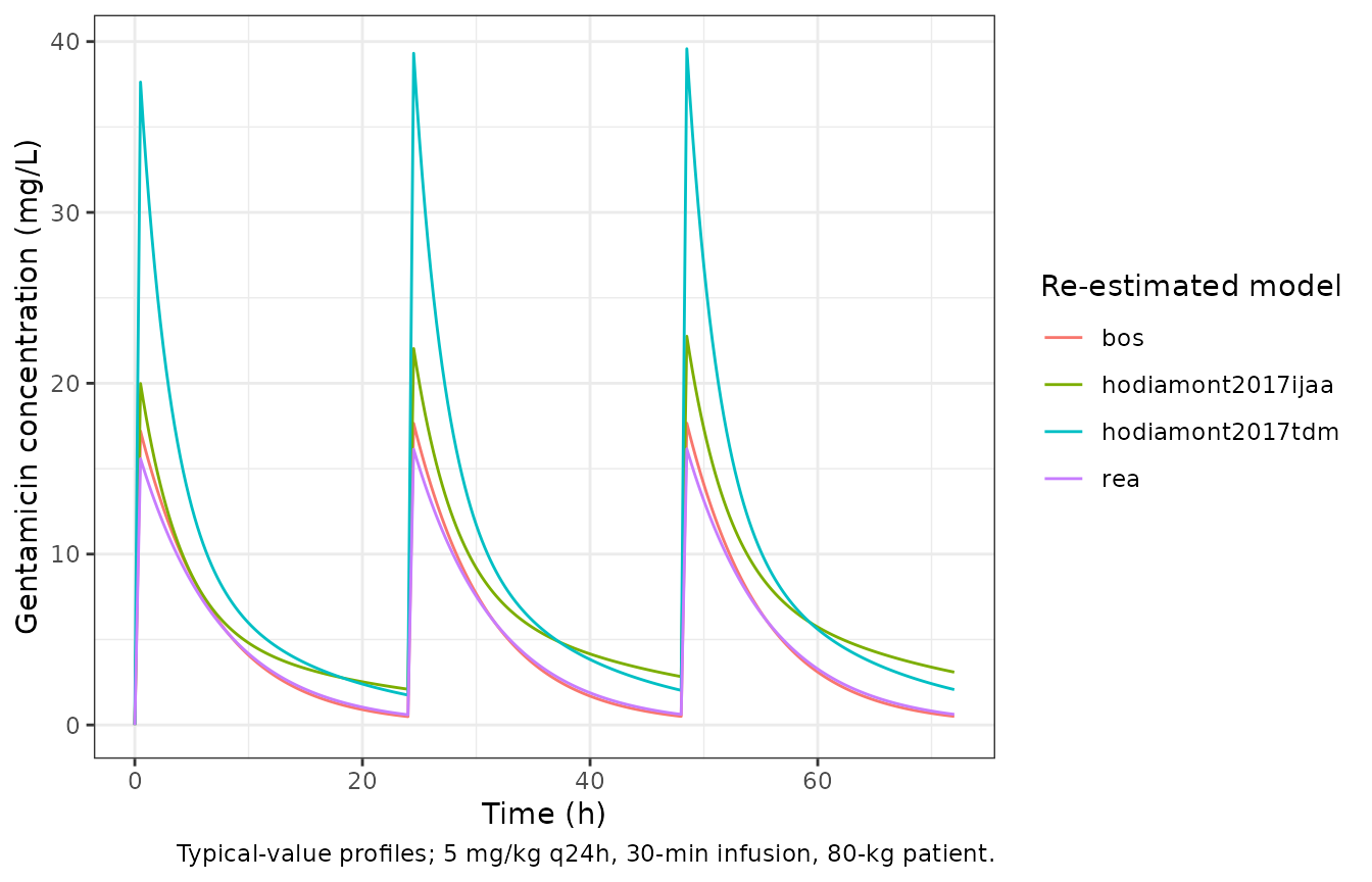
Replicating the dosing simulations (Tables S5 to S7)
Duong et al. simulated the re-estimated Rea model to find the probability that the peak after the third dose reaches eight or ten times the MIC (Tables S5 and S6). They also simulated the fraction of troughs before the fourth dose below 1 or 0.5 mg/L (Table S7). The simulations used the study patients’ own covariates. The spread of the published attainment across MIC values is only reproduced when residual error is added to the IIV. For 3 mg/kg q24h, Table S5 gives 62.3%, 13.3% and 0.5% at MIC 1, 2 and 4 mg/L. A 1000-subject check by the maintainers gave about 70%, 12% and 0.2% with residual error, but 85%, 5% and 0% with IIV alone. The simulation below therefore includes both. It uses four daily doses (3, 5, 7 and 10 mg/kg/day) at each of the three intervals, with 200 subjects per arm. The peak is taken at the end of a 30-min infusion of the third dose, and the trough just before the fourth dose.
regs <- expand.grid(daily = c(3, 5, 7, 10), tau = c(8, 12, 24))
pta_ev <- bind_rows(lapply(seq_len(nrow(regs)), function(i) {
  dose_mgkg <- regs$daily[i] * regs$tau[i] / 24
  doses <- expand.grid(id = cohort$id, k = 0:3)
  dosing <- data.frame(
    id = doses$id, time = doses$k * regs$tau[i],
    amt = dose_mgkg * cohort$WT[doses$id], evid = 1L
  )
  dosing$rate <- dosing$amt / 0.5
  obs <- data.frame(
    id = rep(cohort$id, each = 2),
    time = rep(c(2 * regs$tau[i] + 0.5, 3 * regs$tau[i]), n_sub),
    amt = 0, rate = 0, evid = 0L
  )
  out <- bind_rows(dosing, obs)
  out$arm <- i
  out
})) |>
  mutate(cmt = "central", subj = id, id = (arm - 1L) * n_sub + subj) |>
  arrange(id, time, desc(evid))
idx <- pta_ev$subj
pta_ev$WT <- cohort$WT[idx]
pta_ev$CRCL <- cohort$eGFR[idx]
pta_sim <- rxode2::rxSolve(mods$rea, pta_ev, returnType = "data.frame")
#> ℹ parameter labels from comments will be replaced by 'label()'
stopifnot(!anyNA(pta_sim$sim))
pk3 <- pta_sim |>
  mutate(arm = (id - 1L) %/% n_sub + 1L) |>
  group_by(arm, id) |>
  summarise(
    cmax = sim[time == min(time)],
    ctrough = sim[time == max(time)],
    .groups = "drop"
  ) |>
  left_join(regs |> mutate(arm = row_number()), by = "arm")
stopifnot(nrow(pk3) == nrow(regs) * n_sub)
mics <- c(0.25, 0.5, 1, 2, 4)
pta_sim_tab <- bind_rows(lapply(mics, function(m) {
  pk3 |>
    group_by(daily, tau) |>
    summarise(
      `Cmax/MIC > 8` = 100 * mean(cmax / m > 8),
      `Cmax/MIC > 10` = 100 * mean(cmax / m > 10),
      .groups = "drop"
    ) |>
    mutate(MIC = m)
})) |>
  pivot_longer(c(`Cmax/MIC > 8`, `Cmax/MIC > 10`), names_to = "target", values_to = "simulated")

# Published values for the simulated regimens, Tables S5 (target 8) and S6
# (target 10). Rows are MIC 0.25, 0.5, 1, 2 and 4 mg/L; within each daily dose
# the order is q8h, q12h, q24h.
pub_s5 <- list(
  `3` = c(91.6, 94.6, 99.2, 57.3, 75.7, 93.8, 8.6, 20.9, 62.3, 0.1, 0.3, 13.3, 0, 0, 0.5),
  `5` = c(97.7, 98.1, 99.4, 87.3, 93.5, 98.0, 41.0, 64.8, 90.5, 2.6, 13.2, 51.3, 0, 0, 6.5),
  `7` = c(99.0, 99.4, 100.0, 95.5, 97.5, 99.1, 69.2, 82.5, 96.4, 14.5, 33.5, 74.8, 0.4, 2.5, 22.5),
  `10` = c(99.1, 99.5, 99.7, 97.4, 98.8, 99.5, 87.4, 94.1, 98.6, 37.7, 62.2, 89.5, 2.7, 11.3, 49.4)
)
pub_s6 <- list(
  `3` = c(84.7, 91.3, 98.2, 37.5, 60.1, 89.2, 2.1, 8.5, 46.2, 0, 0, 5.9, 0, 0, 0),
  `5` = c(92.6, 97.4, 99.4, 61.1, 88.4, 97.4, 22.4, 44.7, 82.0, 0.2, 4.3, 32.8, 0, 0, 2.0),
  `7` = c(97.8, 98.9, 99.8, 85.7, 96.0, 98.2, 38.7, 73.0, 92.5, 2.2, 18.2, 60.1, 0, 0.8, 11.3),
  `10` = c(98.9, 99.5, 99.7, 96.2, 98.3, 99.1, 76.0, 89.2, 97.1, 20.5, 43.7, 80.6, 0.4, 3.9, 31.6)
)
pub_long <- function(lst, target) {
  bind_rows(lapply(names(lst), function(d) {
    data.frame(
      daily = as.numeric(d),
      MIC = rep(mics, each = 3),
      tau = rep(c(8, 12, 24), times = length(mics)),
      published = lst[[d]],
      target = target
    )
  }))
}
pub_tab <- bind_rows(pub_long(pub_s5, "Cmax/MIC > 8"), pub_long(pub_s6, "Cmax/MIC > 10"))
pta_cmp <- inner_join(pta_sim_tab, pub_tab, by = c("daily", "tau", "MIC", "target")) |>
  mutate(diff = simulated - published)
stopifnot(nrow(pta_cmp) == nrow(pub_tab))

pta_cmp |>
  filter(target == "Cmax/MIC > 8") |>
  mutate(
    Regimen = sprintf("%g mg/kg/day q%gh", daily, tau),
    simulated = round(simulated, 1)
  ) |>
  select(Regimen, MIC, simulated, published) |>
  rename(`MIC (mg/L)` = MIC, `Simulated PTA (%)` = simulated, `Table S5 PTA (%)` = published) |>
knitr::kable(caption = "Probability of Cmax/MIC > 8 after the third dose (compare Table S5).")| Regimen | MIC (mg/L) | Simulated PTA (%) | Table S5 PTA (%) |
|---|---|---|---|
| 3 mg/kg/day q8h | 0.25 | 90.5 | 91.6 |
| 3 mg/kg/day q12h | 0.25 | 94.0 | 94.6 |
| 3 mg/kg/day q24h | 0.25 | 100.0 | 99.2 |
| 5 mg/kg/day q8h | 0.25 | 99.0 | 97.7 |
| 5 mg/kg/day q12h | 0.25 | 99.5 | 98.1 |
| 5 mg/kg/day q24h | 0.25 | 98.5 | 99.4 |
| 7 mg/kg/day q8h | 0.25 | 99.0 | 99.0 |
| 7 mg/kg/day q12h | 0.25 | 99.0 | 99.4 |
| 7 mg/kg/day q24h | 0.25 | 99.0 | 100.0 |
| 10 mg/kg/day q8h | 0.25 | 98.5 | 99.1 |
| 10 mg/kg/day q12h | 0.25 | 99.5 | 99.5 |
| 10 mg/kg/day q24h | 0.25 | 99.0 | 99.7 |
| 3 mg/kg/day q8h | 0.50 | 65.5 | 57.3 |
| 3 mg/kg/day q12h | 0.50 | 74.5 | 75.7 |
| 3 mg/kg/day q24h | 0.50 | 97.0 | 93.8 |
| 5 mg/kg/day q8h | 0.50 | 92.5 | 87.3 |
| 5 mg/kg/day q12h | 0.50 | 97.0 | 93.5 |
| 5 mg/kg/day q24h | 0.50 | 98.0 | 98.0 |
| 7 mg/kg/day q8h | 0.50 | 95.5 | 95.5 |
| 7 mg/kg/day q12h | 0.50 | 97.5 | 97.5 |
| 7 mg/kg/day q24h | 0.50 | 98.5 | 99.1 |
| 10 mg/kg/day q8h | 0.50 | 98.5 | 97.4 |
| 10 mg/kg/day q12h | 0.50 | 99.5 | 98.8 |
| 10 mg/kg/day q24h | 0.50 | 98.5 | 99.5 |
| 3 mg/kg/day q8h | 1.00 | 8.0 | 8.6 |
| 3 mg/kg/day q12h | 1.00 | 26.0 | 20.9 |
| 3 mg/kg/day q24h | 1.00 | 70.5 | 62.3 |
| 5 mg/kg/day q8h | 1.00 | 47.0 | 41.0 |
| 5 mg/kg/day q12h | 1.00 | 68.0 | 64.8 |
| 5 mg/kg/day q24h | 1.00 | 92.5 | 90.5 |
| 7 mg/kg/day q8h | 1.00 | 74.0 | 69.2 |
| 7 mg/kg/day q12h | 1.00 | 87.0 | 82.5 |
| 7 mg/kg/day q24h | 1.00 | 93.5 | 96.4 |
| 10 mg/kg/day q8h | 1.00 | 85.5 | 87.4 |
| 10 mg/kg/day q12h | 1.00 | 96.0 | 94.1 |
| 10 mg/kg/day q24h | 1.00 | 97.0 | 98.6 |
| 3 mg/kg/day q8h | 2.00 | 0.0 | 0.1 |
| 3 mg/kg/day q12h | 2.00 | 0.5 | 0.3 |
| 3 mg/kg/day q24h | 2.00 | 11.0 | 13.3 |
| 5 mg/kg/day q8h | 2.00 | 4.0 | 2.6 |
| 5 mg/kg/day q12h | 2.00 | 11.5 | 13.2 |
| 5 mg/kg/day q24h | 2.00 | 56.5 | 51.3 |
| 7 mg/kg/day q8h | 2.00 | 19.0 | 14.5 |
| 7 mg/kg/day q12h | 2.00 | 35.5 | 33.5 |
| 7 mg/kg/day q24h | 2.00 | 77.5 | 74.8 |
| 10 mg/kg/day q8h | 2.00 | 38.5 | 37.7 |
| 10 mg/kg/day q12h | 2.00 | 62.0 | 62.2 |
| 10 mg/kg/day q24h | 2.00 | 93.0 | 89.5 |
| 3 mg/kg/day q8h | 4.00 | 0.0 | 0.0 |
| 3 mg/kg/day q12h | 4.00 | 0.0 | 0.0 |
| 3 mg/kg/day q24h | 4.00 | 0.5 | 0.5 |
| 5 mg/kg/day q8h | 4.00 | 0.0 | 0.0 |
| 5 mg/kg/day q12h | 4.00 | 0.0 | 0.0 |
| 5 mg/kg/day q24h | 4.00 | 3.5 | 6.5 |
| 7 mg/kg/day q8h | 4.00 | 0.5 | 0.4 |
| 7 mg/kg/day q12h | 4.00 | 0.0 | 2.5 |
| 7 mg/kg/day q24h | 4.00 | 20.5 | 22.5 |
| 10 mg/kg/day q8h | 4.00 | 2.5 | 2.7 |
| 10 mg/kg/day q12h | 4.00 | 9.5 | 11.3 |
| 10 mg/kg/day q24h | 4.00 | 58.0 | 49.4 |
ggplot(pta_cmp, aes(published, simulated, colour = factor(tau))) +
  geom_abline(linetype = 2) +
  geom_point() +
  facet_wrap(~target) +
  coord_equal(xlim = c(0, 100), ylim = c(0, 100)) +
  labs(
    x = "Published PTA (%) (Tables S5 and S6)", y = "Simulated PTA (%)",
    colour = "Interval (h)",
    caption = "Replicates Tables S5 and S6 / Figure 2 of Duong 2022 for 3, 5, 7 and 10 mg/kg/day."
  ) +
  theme_bw()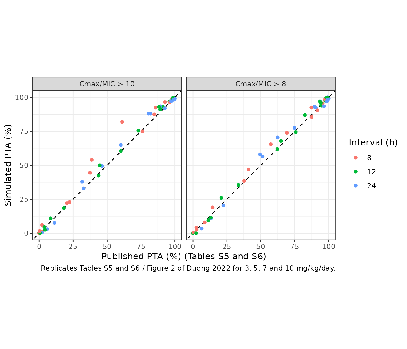
pta_summary <- pta_cmp |>
  summarise(
    cells = n(),
    median_abs_diff = median(abs(diff)),
    p90_abs_diff = unname(quantile(abs(diff), 0.9))
  )
knitr::kable(pta_summary, digits = 1)| cells | median_abs_diff | p90_abs_diff |
|---|---|---|
| 120 | 1.1 | 5.2 |
# Each simulated PTA is a binomial proportion over 200 subjects: SE at most
# 3.5 percentage points, so a cell differs from the model-true value by up to
# about 7 points by chance alone. The cohort is also a reconstruction of the
# 87 patients, not the patients themselves. The gate therefore tests the centre
# and the 90th percentile of |difference| over 120 cells. Realised: median 1.1
# and 90th percentile 5.2 points; the bounds leave about 3x headroom for a
# different cohort draw. Halving V or doubling clearance moves the mid-range
# cells by 30-60 points, which these bounds cannot absorb.
stopifnot(
  pta_summary$cells == 120L,
  pta_summary$median_abs_diff < 4,
  pta_summary$p90_abs_diff < 15
)
The pre-fourth-dose troughs below 1 and 0.5 mg/L at the q24h interval are compared with Table S7:
pub_s7 <- data.frame(
  daily = c(3, 5, 7, 10),
  `<1 published` = c(70.3, 56.5, 49.3, 39.6),
  `<0.5 published` = c(47.0, 38.5, 33.1, 25.9),
  check.names = FALSE
)
trough_cmp <- pk3 |>
  filter(tau == 24) |>
  group_by(daily) |>
  summarise(`<1 simulated` = 100 * mean(ctrough < 1), `<0.5 simulated` = 100 * mean(ctrough < 0.5)) |>
  left_join(pub_s7, by = "daily")
trough_cmp |>
  rename(`Dose (mg/kg q24h)` = daily) |>
knitr::kable(digits = 1, caption = "Percentage of troughs before the fourth dose below 1 or 0.5 mg/L (compare Table S7).")| Dose (mg/kg q24h) | <1 simulated | <0.5 simulated | <1 published | <0.5 published |
|---|---|---|---|---|
| 3 | 63.5 | 50.5 | 70.3 | 47.0 |
| 5 | 61.0 | 43.5 | 56.5 | 38.5 |
| 7 | 55.0 | 35.0 | 49.3 | 33.1 |
| 10 | 45.0 | 28.0 | 39.6 | 25.9 |
The trough fractions are reported, not gated. They depend strongly on the additive residual error (0.279 mg/L) near the 0.5 and 1 mg/L thresholds, and that error comes from the bootstrap means rather than a final estimate.
NCA of a single dose (PKNCA)
The paper publishes no NCA results. To give users comparable summaries of the four models, each one simulates the virtual cohort (with IIV) after a single 5 mg/kg 30-min infusion, and PKNCA computes Cmax, AUC0-24 and half-life.
obs_times <- c(0, 0.25, 0.5, 0.75, 1, 1.5, 2, 3, 4, 6, 8, 10, 12, 16, 20, 24)
nca_ev <- bind_rows(
  data.frame(id = cohort$id, time = 0, amt = 5 * cohort$WT, rate = 10 * cohort$WT, evid = 1L),
  data.frame(id = rep(cohort$id, each = length(obs_times)), time = rep(obs_times, n_sub), amt = 0, rate = 0, evid = 0L)
) |>
  mutate(cmt = "central") |>
  arrange(id, time, desc(evid))
nca_sim <- bind_rows(lapply(names(mods), function(k) {
  s <- rxode2::rxSolve(mods[[k]], add_cov(nca_ev, k), returnType = "data.frame")
  data.frame(model = k, id = s$id, time = s$time, Cc = s$Cc)
}))
#> ℹ parameter labels from comments will be replaced by 'label()'
#> ℹ parameter labels from comments will be replaced by 'label()'
#> ℹ parameter labels from comments will be replaced by 'label()'
stopifnot(!anyNA(nca_sim$Cc))
dose_df <- data.frame(id = cohort$id, time = 0, dose = 5 * cohort$WT) |>
  tidyr::crossing(model = names(mods))
conc_obj <- PKNCA::PKNCAconc(nca_sim |> filter(!is.na(Cc)), Cc ~ time | model + id)
dose_obj <- PKNCA::PKNCAdose(dose_df, dose ~ time | model + id)
intervals <- data.frame(start = 0, end = 24, cmax = TRUE, tmax = TRUE, auclast = TRUE, half.life = TRUE)
nca_res <- PKNCA::pk.nca(PKNCA::PKNCAdata(conc_obj, dose_obj, intervals = intervals))
nca_tab <- as.data.frame(nca_res) |>
  filter(PPTESTCD %in% c("cmax", "auclast", "half.life")) |>
  group_by(model, PPTESTCD) |>
  summarise(median = median(PPORRES, na.rm = TRUE), .groups = "drop") |>
  pivot_wider(names_from = PPTESTCD, values_from = median)
nca_tab |>
  rename(
    `Re-estimated model` = model, `Cmax (mg/L)` = cmax,
    `AUC0-24 (mg*h/L)` = auclast, `t1/2 (h)` = half.life
  ) |>
knitr::kable(digits = 2, caption = "Median single-dose NCA, 5 mg/kg, n = 200 per model.")| Re-estimated model | AUC0-24 (mg*h/L) | Cmax (mg/L) | t1/2 (h) |
|---|---|---|---|
| bos | 112.19 | 17.80 | 4.47 |
| hodiamont2017ijaa | 140.61 | 21.79 | 14.68 |
| hodiamont2017tdm | 200.51 | 37.67 | 8.77 |
| rea | 115.35 | 15.34 | 5.03 |
The re-estimated Rea and Bos models (V about 22 L at 70 kg) and the Hodiamont IJAA model (V1 23.9 L) give median peaks of roughly 15-22 mg/L after 5 mg/kg. The Hodiamont TDM re-estimate has a small central volume (V1 8.67 L) and gives a much higher end-of-infusion peak. This matches Duong et al.’s observation that the re-estimated Hodiamont TDM volume was about half the original value.
Assumptions and deviations
-
What is packaged. Only the four re-estimated models
are packaged here, one file each, because each was fitted separately.
The original parameter sets in Table S1 are the source authors’ models
and belong in extractions of those papers. Hodiamont 2017 (Ther Drug
Monit) is packaged as
Hodiamont_2017_gentamicin. -
Residual error of the re-estimated models. Table S2
drops the residual-error columns that Table S1 carries, and the text
says only that “the PK parameters and interindividual variability were
re-estimated”.
- Rea: the only reported values are the Table S4 bootstrap means (proportional 34.4%, additive 0.279 mg/L), which are used here. The Table S4 bootstrap mean for thetaCL,a (9.74, 95% CI 9.62-9.87) does not contain the Table S2 estimate (9.31), so the bootstrap means are not identical to the final estimates.
- Bos and Hodiamont TDM: the original residual errors from Table S1 are carried forward.
- Hodiamont IJAA: neither Table S1 nor Table S2 reports a magnitude
for its proportional error, so
propSdis fixed to 0. Supply a value before using this model for stochastic simulation.
-
Hodiamont IJAA V1. Table S2’s theta column and
Table S3 both give 23.9 L and CL 2.12 L/h. The equation column of the
same table prints
CL = 2.11 x ...andV1 = 21.2 x ..., which matches the original Table S1 V1. The text says both CL and total volume rose after re-estimation. Only 23.9 L satisfies that (total 42.0 L vs 39.6 L originally); 21.2 L would give 39.3 L. So 23.9 L and 2.12 L/h are used. - Rea IIV. Table S2 gives 36.9% (CL,a), 18.3% (CL,b) and 28.8% (V). Table S3 instead lists 60.7% (CL) and 42.8% (V). The Table S4 bootstrap means (35.9%, 16.6% and 27.9%) agree with Table S2, so Table S2 is used.
- Coefficients printed unchanged from Table S1 are encoded as fixed: the Rea Hill exponent 1.2 and the Hodiamont IJAA albumin exponent -0.833. Allometric exponents (0.75, 1) are fixed as well. The Bos CrCl slope changed (0.0091 to 0.00925) and its centring moved from 74 to 92 mL/min, so it is treated as estimated.
-
Hodiamont TDM structure. The original Hodiamont
2017 TDM paper retained no body-weight covariate, and its final model
has a CL-V1 correlation (see
Hodiamont_2017_gentamicin). Duong et al. specified the model with allometric weight scaling on CL, Q and V1 and no correlation, and re-estimated it in that form. It is packaged as Duong et al. specified it. - Covariates missing from the Quebec data. Height was not recorded, so ideal body weight could not be computed. Albumin was recorded only at IUCPQ. By the paper’s stated rule, such covariates take the model’s typical value (IBW 70 kg, albumin 22 g/L). The re-estimated IBW coefficients, and the albumin effect for HSCM patients, are therefore not informed by Quebec data.
- Renal function. eGFR is the four-variable MDRD equation as printed (Methods Eq. 1), labelled mL/min without BSA de-normalisation. CrCl is the Cockcroft-Gault equation with SCr in umol/L (Eq. 2) on total body weight.
-
Omega scale. IIV is reported as CV% with no
definition; the standard
omega^2 = log(1 + CV^2)is used. - Simulation design. Neither the infusion duration nor the timing of the peak is stated. A 30-min infusion and an end-of-infusion peak are assumed. The virtual cohort replaces the 87 study patients, with no patient coded as Black and SCr chosen to match the published eGFR and CrCl means.