Model and source
#> ℹ parameter labels from comments will be replaced by 'label()'Citation: Xu D, Li H, Heitner SB, Jacoby DL, Kupfer S, German P, Lutz J. Toward a Quantitative Understanding of Aficamten Clinical Pharmacology: Population Pharmacokinetic Modeling. CPT Pharmacometrics Syst Pharmacol. 2025;14(12):1982-1992. doi:10.1002/psp4.70099
Description: Two-compartment population PK model for aficamten with first-order absorption and a formulation-dependent lag time in healthy participants and participants with obstructive hypertrophic cardiomyopathy (Xu 2025)
Article: https://doi.org/10.1002/psp4.70099
Supporting Information Data S1 (NONMEM control file of the final model) and Data S2 (supplemental methods, Tables S1-S5, Figures S1-S6) are distributed with the open-access article at the DOI above.
Aficamten is a cardiac myosin inhibitor developed as a chronic oral treatment for hypertrophic cardiomyopathy. Xu 2025 pooled nine clinical studies into a single population PK analysis and reported a two-compartment model with linear elimination, first-order absorption, and a formulation-dependent absorption lag time.
Population
The analysis dataset comprised 9963 aficamten plasma concentrations from 447 participants across nine studies (Xu 2025 Table S1, Table S3): 264 healthy participants in seven phase 1 studies, 41 participants with obstructive hypertrophic cardiomyopathy (oHCM) from the phase 2 REDWOOD-HCM trial (NCT04219826), and 142 participants with oHCM from the pivotal phase 3 SEQUOIA-HCM trial (NCT05186818). Aficamten was given orally as a capsule or a tablet, either as a single dose of 1-75 mg or as multiple once-daily doses of 5-30 mg. Phase 1 studies used intensive sampling; the phase 2 and phase 3 studies used sparse sampling.
Baseline demographics (Xu 2025 Table S5): median age 43 years (range 18-83), median body weight 77.2 kg (range 47.0-156), 39.4% female, 71.1% White, 13.4% Asian, 11.2% Black or African American. Renal function was normal in 83.7%, mildly impaired in 13.4%, and moderately impaired in 2.9%. Concentrations below the 1 ng/mL lower limit of quantitation (n = 373) were excluded from the analysis, as were participants with hepatic impairment and participants with non-obstructive HCM.
The same information is available programmatically via the model’s
population metadata
(rxode2::rxode(readModelDb("Xu_2025_aficamten"))$population).
Source trace
Every ini() entry in
inst/modeldb/specificDrugs/Xu_2025_aficamten.R carries an
in-file comment naming its source location. They are collected here for
review.
| Equation / parameter | Value | Source location |
|---|---|---|
lcl (CL/F) |
2.62 L/h | Table 1; Figure S3 |
lvc (Vc/F) |
18.1 L | Table 1; Figure S3 |
lq (Q/F) |
57.6 L/h | Table 1; Figure S3 |
lvp (Vp/F) |
295 L | Table 1; Figure S3 |
lka (Ka) |
0.337 1/h | Table 1 (Figure S3 prints 0.373 – see Errata) |
ltlag_tab |
0.229 h | Table 1 “Tlag of tablets”; Figure S3 |
ltlag_cap |
0.248 h | Table 1 “Tlag of capsule”; Figure S3 |
lfdepot (F1 reference) |
1 (fixed) | Data S1 control stream, TVF1 = 1 * (...)
|
e_wt_cl_q |
0.586 | Table 1 “WT on CL/F and Q/F”; Figure S3 |
e_wt_vc_vp |
0.882 | Table 1 “WT on Vc/F and Vp/F”; Figure S3 |
e_dis_healthy_cl |
0.356 | Table 1 “Healthy participants on CL/F”; Figure S3 |
e_sexf_cl |
-0.128 | Table 1 “Sex female on CL/F”; Figure S3 |
e_dis_healthy_vp |
0.266 | Table 1 “Healthy participants on Vp/F”; Figure S3 |
e_sexf_vp |
-0.193 | Table 1 “Sex female on Vp/F”; Figure S3 |
e_fed_ka |
0.170 | Table 1 “Fasted on Ka”; Figure S3 |
e_fed_highfat_ka |
-0.365 | Table 1 “High fat meal on Ka”; Figure S3 |
e_fed_highfat_tlag |
0.115 | Table 1 “High fat meal on Tlag”; Figure S3 |
e_fed_highfat_fdepot |
0.0687 | Table 1 “High fat meal on F1” (Figure S3 prints 0.0686) |
etalcl |
0.0793 (28.7% CV) | Table 1 |
etalvc |
2.35 (308% CV) | Table 1 |
etalvp |
0.041 (20.5% CV) | Table 1 |
etalka |
0.329 (62.4% CV) | Table 1 |
| IIV on Q/F | fixed to 0 (omitted) | Data S1 control stream, $OMEGA 0 FIX ; BSVQ/F
|
expSd |
sqrt(0.0414) = 0.2035 | Table 1 “delta^2 (log-additive)” |
| 2-compartment ODEs, first-order absorption with lag | n/a | Section 3.1.1; Data S1 ($SUBROUTINE ADVAN4 TRANS4) |
Proportional (1 + theta * Q) categorical covariate
form |
n/a | Figure S1; Figure S3 |
Power ((X / M(X))^theta) continuous covariate form,
M(WT) = 80 kg
|
n/a | Figure S1; Section 2.3.2; Figure S3 |
Concentration scaling Cc = 1000 * central / vc
|
n/a | Data S1,
S2 = V2/1000 ;Scaling factor conc ng/mL, dose in mg
|
Virtual cohort
Original observed data are not publicly available. The simulations below use virtual cohorts whose covariate distributions approximate the published trial demographics (Xu 2025 Table S5).
tau <- 24  # once-daily dosing interval (h)

# Observation grid over one dosing interval: dense through the absorption
# phase so Tmax and Cmax are resolved, coarser across the flat tail.
obs_grid <- sort(unique(c(seq(0, 4, by = 0.05), seq(4, tau, by = 0.5))))

# Build a steady-state event table from a per-subject covariate frame. The dose
# record carries `ss = 1` with `ii = tau`, so rxode2 places each subject at
# exact steady state analytically rather than by simulating a long dose train.
# This matters here: the published IIV on Vc/F is 308% CV, which gives a tail of
# subjects with terminal half-lives beyond 700 h. Those subjects would still be
# accumulating after 40 daily doses, which is the paper's own observation that
# ~5% of participants with oHCM need until day 33 to reach steady state
# (Xu 2025 Table 2 and Section 3.2.1). `ss = 1` removes that approximation
# entirely, so the structural checks below hold per subject rather than on
# average. `id_offset` keeps IDs disjoint when cohorts are bind_rows()-ed.
make_ss_events <- function(covs, dose, id_offset = 0L, grid = obs_grid) {
  covs$id <- id_offset + seq_len(nrow(covs))
  dosing <- covs |>
    dplyr::mutate(time = 0, amt = dose, evid = 1L, cmt = "depot",
                  ss = 1L, ii = tau)
  obs <- covs |>
    tidyr::crossing(time = grid) |>
    dplyr::mutate(amt = NA_real_, evid = 0L, cmt = "central",
                  ss = 0L, ii = 0)
  dplyr::bind_rows(dosing, obs) |>
    dplyr::arrange(id, time, dplyr::desc(evid))
}

# Reference covariate set: the Figure 4 base case -- a male participant with
# oHCM weighing 80 kg, given a 15 mg tablet, with or without food.
base_covs <- tibble::tibble(
  WT = 80, SEXF = 0, DIS_HEALTHY = 0,
  FORM_CAPSULE = 0, FED = 1, FED_HIGHFAT = 0
)
Isolated-covariate scenarios (Figure 4)
scenarios <- dplyr::bind_rows(
  base_covs |> dplyr::mutate(scenario = "Base"),
  base_covs |> dplyr::mutate(SEXF = 1, WT = 56, scenario = "Female + WT 5%ile (56kg)"),
  base_covs |> dplyr::mutate(WT = 56, scenario = "WT 5%ile (56kg)"),
  base_covs |> dplyr::mutate(WT = 114, scenario = "WT 95%ile (114kg)"),
  base_covs |> dplyr::mutate(SEXF = 1, scenario = "Female"),
  base_covs |> dplyr::mutate(FED_HIGHFAT = 1, scenario = "High Fat Meal"),
  base_covs |> dplyr::mutate(SEXF = 1, WT = 114, scenario = "Female + WT 95%ile (114kg)")
)
ev_fig4 <- make_ss_events(scenarios, dose = 15)
Disease-status cohorts (Table 2)
Body weight is drawn from a log-normal distribution truncated to the published range, with the log-scale median set to the published median and the log-scale SD chosen so the published minimum and maximum sit near the tails of a cohort of the published size. Sex is drawn as a Bernoulli variable at the published female percentage. These distributional choices are assumptions – Xu 2025 reports only medians, ranges, and percentages (Table S5).
set.seed(20250817)
n_arm <- 200L  # <= 200 participants per arm

draw_wt <- function(n, median_wt, lo, hi, sdlog) {
  wt <- stats::rlnorm(n, meanlog = log(median_wt), sdlog = sdlog)
  pmin(pmax(wt, lo), hi)
}

healthy_covs <- base_covs[rep(1L, n_arm), ] |>
  dplyr::mutate(
    DIS_HEALTHY = 1,
    WT   = draw_wt(n_arm, 74.5, 48.2, 108, 0.14),
    SEXF = stats::rbinom(n_arm, 1L, 0.371),
    cohort = "Healthy"
  )
ohcm_covs <- base_covs[rep(1L, n_arm), ] |>
  dplyr::mutate(
    DIS_HEALTHY = 0,
    WT   = draw_wt(n_arm, 80.0, 47.0, 156, 0.21),
    SEXF = stats::rbinom(n_arm, 1L, 0.426),
    cohort = "oHCM"
  )

ev_cohorts <- dplyr::bind_rows(
  make_ss_events(healthy_covs, dose = 15, id_offset = 0L),
  make_ss_events(ohcm_covs,    dose = 15, id_offset = 1000L)
)
stopifnot(!anyDuplicated(ev_cohorts[, c("id", "time", "evid")]))
Simulation
mod <- readModelDb("Xu_2025_aficamten")
mod_typical <- rxode2::zeroRe(mod)
#> ℹ parameter labels from comments will be replaced by 'label()'

# With `ss = 1` the returned `time` is already measured from the steady-state
# dose, so `time_rel` (time after that dose) is simply `time`.
sim_fig4 <- rxode2::rxSolve(
  mod_typical, events = ev_fig4, keep = c("scenario", "WT", "SEXF", "FED_HIGHFAT"),
  returnType = "data.frame",
  # steady-state searches for long-half-life subjects exceed the default step budget
  maxsteps = 1e6
) |>
  dplyr::mutate(time_rel = time)
#> ℹ omega/sigma items treated as zero: 'etalcl', 'etalvc', 'etalvp', 'etalka'
#> Warning: multi-subject simulation without without 'omega'

sim_cohorts <- rxode2::rxSolve(
  mod, events = ev_cohorts, keep = c("cohort", "WT", "SEXF", "DIS_HEALTHY"),
  returnType = "data.frame",
  # steady-state searches for long-half-life subjects exceed the default step budget
  maxsteps = 1e6
) |>
  dplyr::mutate(time_rel = time)
#> ℹ parameter labels from comments will be replaced by 'label()'

stopifnot(!anyNA(sim_fig4$Cc), !anyNA(sim_cohorts$Cc), all(sim_cohorts$Cc >= 0))
Structural checks
At steady state the AUC over a dosing interval must equal
Dose / (CL/F) exactly, for every subject, regardless of the
absorption model. This is a per-subject identity rather than a
comparison of summary statistics, so it localises any error in the
clearance path or in the ng/mL scaling.
trapz <- function(x, y) sum(diff(x) * (utils::head(y, -1) + utils::tail(y, -1)) / 2)

ident <- sim_cohorts |>
  dplyr::group_by(id, cohort, cl) |>
  dplyr::summarise(AUCtau = trapz(time_rel, Cc), .groups = "drop") |>
  dplyr::mutate(
    AUC_theory = 15 * 1000 / cl,   # 15 mg -> ug; CL/F in L/h -> ng*h/mL
    pct_err    = 100 * (AUCtau / AUC_theory - 1)
  )

max_ident_err <- max(abs(ident$pct_err))
cat(sprintf("Largest |AUCtau - Dose/CL| error across %d subjects: %.3f%%\n",
            nrow(ident), max_ident_err))
#> Largest |AUCtau - Dose/CL| error across 400 subjects: 0.038%
# Residual error is trapezoidal-integration error on the observation grid, not
# steady-state approximation error: `ss = 1` places every subject exactly.
stopifnot(max_ident_err < 0.1)
Aficamten PK is linear, so steady-state exposure must be strictly proportional to dose within a fixed covariate set.
dose_levels <- c(5, 10, 15, 20)
lin <- lapply(seq_along(dose_levels), function(i) {
  ev <- make_ss_events(base_covs, dose = dose_levels[i], id_offset = i)
  s <- rxode2::rxSolve(mod_typical, events = ev, returnType = "data.frame",
                       # steady-state searches for long-half-life subjects exceed the default step budget
                       maxsteps = 1e6)
  data.frame(dose = dose_levels[i], AUCtau = trapz(s$time, s$Cc))
}) |> dplyr::bind_rows() |>
  dplyr::mutate(AUC_per_mg = AUCtau / dose)
#> ℹ omega/sigma items treated as zero: 'etalcl', 'etalvc', 'etalvp', 'etalka'
#> ℹ omega/sigma items treated as zero: 'etalcl', 'etalvc', 'etalvp', 'etalka'
#> ℹ omega/sigma items treated as zero: 'etalcl', 'etalvc', 'etalvp', 'etalka'
#> ℹ omega/sigma items treated as zero: 'etalcl', 'etalvc', 'etalvp', 'etalka'

knitr::kable(
  lin |> dplyr::rename("Dose (mg)" = dose,
                       "AUCtau (ng*h/mL)" = AUCtau,
                       "AUCtau / dose (ng*h/mL per mg)" = AUC_per_mg),
  digits = 1,
  caption = "Dose-proportionality of steady-state exposure in the Figure 4 base subject."
)| Dose (mg) | AUCtau (ng*h/mL) | AUCtau / dose (ng*h/mL per mg) |
|---|---|---|
| 5 | 1908.4 | 381.7 |
| 10 | 3816.9 | 381.7 |
| 15 | 5725.3 | 381.7 |
| 20 | 7633.7 | 381.7 |
Xu 2025 Table 3 reports steady-state exposures by last titrated dose that are not dose-proportional (AUCtau/dose falls from 530 at 5 mg to 379 ng*h/mL per mg at 20 mg). That is a property of the titration design – dose is titrated to echocardiographic response, so participants who were titrated up are systematically those with lower exposure per mg – not a property of the model, which is exactly linear as shown above.
Replicate published figures
Figure 4 – isolated impact of covariates on steady-state exposure
Figure 4 of Xu 2025 reports the isolated effect of each covariate on steady-state AUCtau, Cmax, and Ctau for a 15 mg once-daily tablet regimen, relative to a base case of a male participant with oHCM weighing 80 kg.
Provenance of the reference values below: the
WT 5%ile (56kg), WT 95%ile (114kg), and
Female rows are quoted verbatim from the article text
(Section 3.2.2), and the base-case AUCtau (5720 ng*h/mL)
and Cmax (241 ng/mL) are printed in the Figure 4 panel
annotations. The remaining values – the two combined sex-plus-weight
rows, the High Fat Meal row, and the base-case
Ctau (213 ng/mL) – were read off the Figure 4
forest panels; Xu 2025 tabulates them nowhere. Two independent
checks confirm the digitisation: the base-case Ctau of 213
ng/mL reproduces the analytic steady-state trough of the published
parameters to three significant figures, and the digitised high-fat-meal
AUCtau shift of +6.9% reproduces the +6.87% implied exactly
by the published F1 coefficient.
exposure <- sim_fig4 |>
  dplyr::group_by(scenario) |>
  dplyr::arrange(time_rel, .by_group = TRUE) |>
  dplyr::summarise(
    AUCtau = trapz(time_rel, Cc),
    Cmax   = max(Cc),
    Ctau   = Cc[which.max(time_rel)],
    .groups = "drop"
  )

base_row <- exposure |> dplyr::filter(scenario == "Base")

published <- tibble::tribble(
  ~scenario,                          ~dAUCtau, ~dCmax, ~dCtau,
  "Female + WT 5%ile (56kg)",             41.0,   47.8,   39.8,
  "WT 5%ile (56kg)",                      23.0,   24.6,   22.0,
  "WT 95%ile (114kg)",                   -18.7,  -19.6,  -18.1,
  "Female",                               14.7,   17.7,   14.7,
  "High Fat Meal",                         6.9,   12.9,    8.4,
  "Female + WT 95%ile (114kg)",           -6.8,   -5.8,   -6.0
)

fig4 <- exposure |>
  dplyr::filter(scenario != "Base") |>
  dplyr::mutate(
    sim_dAUCtau = 100 * (AUCtau / base_row$AUCtau - 1),
    sim_dCmax   = 100 * (Cmax   / base_row$Cmax   - 1),
    sim_dCtau   = 100 * (Ctau   / base_row$Ctau   - 1)
  ) |>
  dplyr::inner_join(published, by = "scenario") |>
  dplyr::select(scenario,
                dAUCtau, sim_dAUCtau,
                dCtau,   sim_dCtau,
                dCmax,   sim_dCmax)
stopifnot(nrow(fig4) == nrow(published))

knitr::kable(
  fig4 |> dplyr::rename(
    "Scenario"                = scenario,
    "AUCtau published (%)"    = dAUCtau,
    "AUCtau simulated (%)"    = sim_dAUCtau,
    "Ctau published (%)"      = dCtau,
    "Ctau simulated (%)"      = sim_dCtau,
    "Cmax published (%)"      = dCmax,
    "Cmax simulated (%)"      = sim_dCmax
  ),
  digits = 1,
  caption = paste(
    "Replicates Figure 4 of Xu 2025: isolated percent change in steady-state",
    "exposure versus the base case (male with oHCM, 80 kg, 15 mg tablet)."
  )
)| Scenario | AUCtau published (%) | AUCtau simulated (%) | Ctau published (%) | Ctau simulated (%) | Cmax published (%) | Cmax simulated (%) |
|---|---|---|---|---|---|---|
| Female | 14.7 | 14.7 | 14.7 | 14.7 | 17.7 | 11.6 |
| Female + WT 5%ile (56kg) | 41.0 | 41.3 | 39.8 | 40.2 | 47.8 | 37.4 |
| Female + WT 95%ile (114kg) | -6.8 | -6.8 | -6.0 | -6.0 | -5.8 | -9.2 |
| High Fat Meal | 6.9 | 6.9 | 8.4 | 8.4 | 12.9 | -0.1 |
| WT 5%ile (56kg) | 23.0 | 23.2 | 22.0 | 22.2 | 24.6 | 23.1 |
| WT 95%ile (114kg) | -18.7 | -18.7 | -18.1 | -18.1 | -19.6 | -18.7 |
The base-case absolute values are reproduced as well:
base_cmp <- tibble::tibble(
  Quantity   = c("AUCtau (ng*h/mL)", "Ctau (ng/mL)", "Cmax (ng/mL)"),
  Published  = c(5720, 213, 241),
  Simulated  = c(base_row$AUCtau, base_row$Ctau, base_row$Cmax)
) |>
  dplyr::mutate(`% diff` = 100 * (Simulated / Published - 1))

knitr::kable(base_cmp, digits = c(0, 0, 1, 1),
caption = "Figure 4 base case, published versus simulated.")| Quantity | Published | Simulated | % diff |
|---|---|---|---|
| AUCtau (ng*h/mL) | 5720 | 5725.3 | 0.1 |
| Ctau (ng/mL) | 213 | 213.3 | 0.2 |
| Cmax (ng/mL) | 241 | 280.8 | 16.5 |
AUCtau and Ctau are reproduced to better than 0.5 percentage points in every scenario and to better than 0.5% in the base case. The Cmax column is not reproduced; see Errata below. The assertions therefore gate AUCtau and Ctau strictly and do not gate Cmax.
Figure 3 – distribution of individual PK parameters
Figure 3 of Xu 2025 shows the distributions of CL/F, total apparent volume (Vc/F + Vp/F), and terminal half-life in each disease cohort.
subj <- sim_cohorts |>
  dplyr::group_by(id, cohort) |>
  dplyr::summarise(cl = dplyr::first(cl), vc = dplyr::first(vc),
                   vp = dplyr::first(vp), q = dplyr::first(q), .groups = "drop") |>
  dplyr::mutate(
    total_v = vc + vp,
    # Terminal (beta) half-life of the two-compartment system
    k10 = cl / vc, k12 = q / vc, k21 = q / vp,
    beta = 0.5 * ((k10 + k12 + k21) -
                    sqrt((k10 + k12 + k21)^2 - 4 * k10 * k21)),
    thalf = log(2) / beta
  )

subj |>
  dplyr::select(cohort, `CL/F (L/h)` = cl, `Total volume (L)` = total_v,
                `T1/2 (h)` = thalf) |>
  tidyr::pivot_longer(-cohort, names_to = "parameter", values_to = "value") |>
  ggplot(aes(value)) +
  geom_histogram(bins = 30, fill = "#f4c7c3", colour = "grey30") +
  facet_grid(cohort ~ parameter, scales = "free") +
  labs(x = NULL, y = "Count",
       caption = "Replicates Figure 3 of Xu 2025 (parameter distributions by cohort).")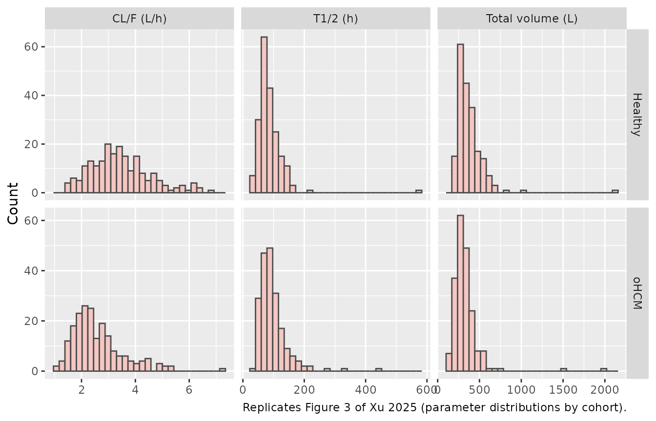
thalf_cmp <- subj |>
  dplyr::group_by(cohort) |>
  dplyr::summarise(
    `T1/2 median (h)` = stats::median(thalf),
    `T1/2 5th (h)`    = stats::quantile(thalf, 0.05),
    `T1/2 95th (h)`   = stats::quantile(thalf, 0.95),
    `Time to steady state, 5 x T1/2 (day)` = stats::median(thalf) * 5 / 24,
    .groups = "drop"
  )
knitr::kable(thalf_cmp, digits = 1, caption = paste(
  "Simulated terminal half-life by cohort. Xu 2025 Table 2 reports a median",
  "(5th, 95th percentile) of 81.4 (60.2, 114) h in healthy participants and",
  "79.9 (54.5, 155) h in participants with oHCM, and a median time to steady",
"state of 17.0 and 16.6 days respectively."))| cohort | T1/2 median (h) | T1/2 5th (h) | T1/2 95th (h) | Time to steady state, 5 x T1/2 (day) |
|---|---|---|---|---|
| Healthy | 78.1 | 45.5 | 143.1 | 16.3 |
| oHCM | 84.6 | 46.4 | 178.0 | 17.6 |
PKNCA validation
Steady-state NCA by disease cohort
sim_nca <- sim_cohorts |>
  dplyr::filter(!is.na(Cc)) |>
  dplyr::select(id, time = time_rel, Cc, cohort)

# Guarantee a time = 0 record per (id, cohort). The simulation grid already
# starts at the last dose, so this is a defensive no-op here.
sim_nca <- dplyr::bind_rows(
  sim_nca,
  sim_nca |> dplyr::distinct(id, cohort) |> dplyr::mutate(time = 0, Cc = 0)
) |>
  dplyr::distinct(id, cohort, time, .keep_all = TRUE) |>
  dplyr::arrange(id, cohort, time)

dose_df <- sim_nca |>
  dplyr::distinct(id, cohort) |>
  dplyr::mutate(time = 0, amt = 15)

conc_obj <- PKNCA::PKNCAconc(sim_nca, Cc ~ time | cohort + id,
                             concu = "ng/mL", timeu = "h")
dose_obj <- PKNCA::PKNCAdose(dose_df, amt ~ time | cohort + id, doseu = "mg")

intervals_ss <- data.frame(
  start = 0, end = tau,
  cmax = TRUE, tmax = TRUE, cmin = TRUE, auclast = TRUE, cav = TRUE
)
nca_ss <- PKNCA::pk.nca(PKNCA::PKNCAdata(conc_obj, dose_obj,
                                         intervals = intervals_ss))
Single-dose NCA for terminal half-life
Steady-state profiles over a single dosing interval carry no terminal phase, so half-life is estimated from a separate single-dose simulation of the same cohorts sampled to 408 h (the schedule of the phase 1 food-effect study, Table S1), truncated at the published 1 ng/mL lower limit of quantitation.
sd_grid <- sort(unique(c(seq(0, 12, by = 0.5), seq(12, 48, by = 2),
                         seq(48, 408, by = 12))))
make_sd_events <- function(covs, dose, id_offset = 0L) {
  covs$id <- id_offset + seq_len(nrow(covs))
  dplyr::bind_rows(
    covs |> dplyr::mutate(time = 0, amt = dose, evid = 1L, cmt = "depot"),
    covs |> tidyr::crossing(time = sd_grid) |>
      dplyr::mutate(amt = NA_real_, evid = 0L, cmt = "central")
  ) |> dplyr::arrange(id, time, dplyr::desc(evid))
}
ev_sd <- dplyr::bind_rows(
  make_sd_events(healthy_covs, dose = 20, id_offset = 0L),
  make_sd_events(ohcm_covs,    dose = 20, id_offset = 1000L)
)
sim_sd <- rxode2::rxSolve(mod, events = ev_sd, keep = "cohort",
                          returnType = "data.frame") |>
  dplyr::filter(!is.na(Cc), Cc >= 1)   # truncate at the 1 ng/mL LLOQ

conc_sd <- PKNCA::PKNCAconc(
  sim_sd |> dplyr::select(id, time, Cc, cohort),
  Cc ~ time | cohort + id, concu = "ng/mL", timeu = "h"
)
dose_sd <- PKNCA::PKNCAdose(
  sim_sd |> dplyr::distinct(id, cohort) |> dplyr::mutate(time = 0, amt = 20),
  amt ~ time | cohort + id, doseu = "mg"
)
nca_sd <- PKNCA::pk.nca(PKNCA::PKNCAdata(
  conc_sd, dose_sd,
  intervals = data.frame(start = 0, end = Inf, half.life = TRUE)
))
Comparison against published NCA
Xu 2025 Table 2 reports AUCtau, Cmax, and Ctau as arithmetic
means and half-life as a median.
ncaComparisonTable() aggregates per-subject values by
median, so the simulated values are pre-aggregated with the matching
statistic before comparison rather than letting the default apply.
ss_res <- as.data.frame(nca_ss$result) |>
  dplyr::filter(PPTESTCD %in% c("auclast", "cmax", "cmin"))

sim_wide <- ss_res |>
  dplyr::group_by(cohort, PPTESTCD) |>
  dplyr::summarise(value = mean(PPORRES), .groups = "drop") |>
  tidyr::pivot_wider(names_from = PPTESTCD, values_from = value) |>
  dplyr::left_join(
    as.data.frame(nca_sd$result) |>
      dplyr::filter(PPTESTCD == "half.life") |>
      dplyr::group_by(cohort) |>
      dplyr::summarise(half.life = stats::median(PPORRES), .groups = "drop"),
    by = "cohort"
  )

published_nca <- tibble::tribble(
  ~cohort,    ~auclast, ~cmax, ~cmin, ~half.life,
  "Healthy",      4770,   206,   176,       81.4,
  "oHCM",         6420,   278,   242,       79.9
)

cmp <- nlmixr2lib::ncaComparisonTable(
  simulated = as.data.frame(sim_wide),
  reference = as.data.frame(published_nca),
  by        = "cohort",
  units     = c(auclast = "ng*h/mL", cmax = "ng/mL",
                cmin = "ng/mL", half.life = "h"),
  tolerance_pct = 20
)

knitr::kable(
  cmp,
  caption = paste(
    "Simulated versus published steady-state NCA after 15 mg once daily",
    "(Xu 2025 Table 2). AUCtau is compared as auclast over the 0-24 h",
    "steady-state interval and Ctau as cmin. * differs by more than 20%."
  ),
  align = c("l", "l", "r", "r", "r")
)| NCA parameter | cohort | Reference | Simulated | % diff |
|---|---|---|---|---|
| Cmax (ng/mL) | Healthy | 206 | 248 | +20.4%* |
| Cmax (ng/mL) | oHCM | 278 | 311 | +11.9% |
| Cmin (ng/mL) | Healthy | 176 | 179 | +1.7% |
| Cmin (ng/mL) | oHCM | 242 | 245 | +1.3% |
| AUClast (ng*h/mL) | Healthy | 4770 | 4830 | +1.4% |
| AUClast (ng*h/mL) | oHCM | 6420 | 6480 | +1.0% |
| t½ (h) | Healthy | 81.4 | 84 | +3.1% |
| t½ (h) | oHCM | 79.9 | 91.4 | +14.4% |
attr(cmp, "footnote")
#> [1] "* differs from reference by more than ±20%."
Simulated AUCtau and Ctau land within about 1.5% of the published means in both cohorts. The only row that exceeds the 20% tolerance is healthy-cohort Cmax (+20.4%); Cmax is high in the oHCM arm too (+11.9%) but stays under the flag. This is the same discrepancy seen in the Figure 4 base case and is discussed in the Errata: the published Cmax column cannot be reproduced from the published parameters, and the paper’s own high-fat-meal effect shows the column to be internally inconsistent. No parameter was adjusted to close the gap.
The oHCM half-life is also high (+14.4%, within tolerance). That is expected rather than anomalous: Xu 2025 derived Table 2 from post-hoc Empirical Bayes estimates, whose Vc/F and Vp/F carried 22.6% and 28.7% shrinkage, while this vignette draws fresh random effects from the full reported OMEGA. Shrunk estimates give a narrower volume distribution and hence a shorter median half-life in the tail-heavy oHCM arm.
The ratio Xu 2025 reports in Table 2 is a geometric mean ratio, whereas the AUCtau / Cmax / Ctau columns of the same table are arithmetic means. The two are not interchangeable at this spread – the published arithmetic means alone give 4770 / 6420 = 0.743 for AUCtau, against the published geometric mean ratio of 0.77 – so the ratio is computed here from per-subject geometric means rather than by reusing the arithmetic means compared above.
geomean <- function(x) exp(mean(log(x)))

gmr <- ss_res |>
  dplyr::group_by(cohort, PPTESTCD) |>
  dplyr::summarise(value = geomean(PPORRES), .groups = "drop") |>
  tidyr::pivot_wider(names_from = cohort, values_from = value) |>
  dplyr::mutate(`Ratio healthy / oHCM` = Healthy / oHCM)

published_gmr <- c(auclast = 0.77, cmax = 0.76, cmin = 0.76)

knitr::kable(
  gmr |>
    dplyr::mutate(Published = published_gmr[PPTESTCD]) |>
    dplyr::rename("NCA parameter" = PPTESTCD,
                  "Geometric mean, healthy" = Healthy,
                  "Geometric mean, oHCM"    = oHCM,
                  "Published ratio"         = Published),
  digits = c(0, 0, 0, 3, 2),
  caption = paste(
    "Healthy / oHCM steady-state exposure ratio, computed as a geometric mean",
    "ratio to match the statistic Xu 2025 Table 2 reports: 0.77 (90% CI 0.73,",
    "0.80) for AUCtau and 0.76 for both Cmax and Ctau."
  )
)| NCA parameter | Geometric mean, healthy | Geometric mean, oHCM | Ratio healthy / oHCM | Published ratio |
|---|---|---|---|---|
| auclast | 4589 | 6139 | 0.748 | 0.77 |
| cmax | 237 | 297 | 0.797 | 0.76 |
| cmin | 168 | 230 | 0.731 | 0.76 |
sim_gmr <- setNames(gmr$`Ratio healthy / oHCM`, gmr$PPTESTCD)Two separate checks follow, because the cohort ratio above confounds two things that are worth gating differently.
1. The structural coefficient, gated exactly. At
matched covariates the healthy/oHCM AUCtau ratio must be exactly
1 / (1 + 0.356), since DIS_HEALTHY enters CL/F
proportionally and AUCtau at steady state is Dose / (CL/F).
This is deterministic, so it is asserted to four decimal places and
would catch any error in e_dis_healthy_cl or in how it is
applied.
matched <- dplyr::bind_rows(
  base_covs |> dplyr::mutate(DIS_HEALTHY = 1, cohort = "Healthy"),
  base_covs |> dplyr::mutate(DIS_HEALTHY = 0, cohort = "oHCM")
)
# steady-state searches for long-half-life subjects exceed the default step budget
sim_matched <- rxode2::rxSolve(mod_typical, events = make_ss_events(matched, dose = 15),
                               keep = "cohort", returnType = "data.frame",
                               maxsteps = 1e6)
#> ℹ omega/sigma items treated as zero: 'etalcl', 'etalvc', 'etalvp', 'etalka'
#> Warning: multi-subject simulation without without 'omega'
matched_auc <- sim_matched |>
  dplyr::group_by(cohort) |>
  dplyr::summarise(AUCtau = trapz(time, Cc), .groups = "drop")
matched_ratio <- matched_auc$AUCtau[matched_auc$cohort == "Healthy"] /
  matched_auc$AUCtau[matched_auc$cohort == "oHCM"]

cat(sprintf("Matched-covariate healthy/oHCM AUCtau ratio: %.5f (expected %.5f)\n",
            matched_ratio, 1 / 1.356))
#> Matched-covariate healthy/oHCM AUCtau ratio: 0.73747 (expected 0.73746)
stopifnot(abs(matched_ratio - 1 / 1.356) < 1e-4)
2. The cohort ratio, gated against its own Monte-Carlo error. The ratio in the table above is estimated from 200 subjects per arm drawn from the reported OMEGA, so it carries sampling noise; at the published IIV that noise is roughly 0.02 on a ratio of 0.77, which is the same size as the discrepancy being tested. Asserting a fixed absolute tolerance would therefore be a seed lottery. The standard error of the log ratio is computed from the simulated data itself and the published value is required to lie within three of them – a check that is stable across seeds but would still fail decisively on a structural error, which would sit many standard errors away.
log_se <- ss_res |>
  dplyr::group_by(PPTESTCD, cohort) |>
  dplyr::summarise(v = stats::var(log(PPORRES)), n = dplyr::n(), .groups = "drop") |>
  dplyr::group_by(PPTESTCD) |>
  dplyr::summarise(se = sqrt(sum(v / n)), .groups = "drop")

gmr_check <- gmr |>
  dplyr::transmute(PPTESTCD,
                   simulated = `Ratio healthy / oHCM`,
                   published = published_gmr[PPTESTCD]) |>
  dplyr::left_join(log_se, by = "PPTESTCD") |>
  dplyr::mutate(n_se = abs(log(simulated / published)) / se)

knitr::kable(
  gmr_check |> dplyr::rename("NCA parameter" = PPTESTCD,
                             "Simulated ratio" = simulated,
                             "Published ratio" = published,
                             "SE of log ratio" = se,
                             "Discrepancy (SE)" = n_se),
  digits = c(0, 3, 2, 4, 2),
  caption = "Cohort geometric mean ratio against its Monte-Carlo standard error."
)| NCA parameter | Simulated ratio | Published ratio | SE of log ratio | Discrepancy (SE) |
|---|---|---|---|---|
| auclast | 0.748 | 0.77 | 0.0329 | 0.90 |
| cmax | 0.797 | 0.76 | 0.0312 | 1.53 |
| cmin | 0.731 | 0.76 | 0.0359 | 1.09 |
stopifnot(
  gmr_check$n_se[gmr_check$PPTESTCD == "auclast"] < 3,
  gmr_check$n_se[gmr_check$PPTESTCD == "cmin"]    < 3
)
The AUCtau and Ctau ratios agree with the published geometric mean
ratios well inside sampling error. This is a sharper check than the
absolute-exposure comparison above, because the ratio cancels most of
the assumed weight and sex distributions and isolates the
DIS_HEALTHY coefficients. Cmax is excluded from both
assertions for the reason given in the Errata.
Steady-state concentration-time profiles
sim_cohorts |>
  dplyr::group_by(cohort, time_rel) |>
  dplyr::summarise(
    Q05 = stats::quantile(Cc, 0.05), Q50 = stats::quantile(Cc, 0.50),
    Q95 = stats::quantile(Cc, 0.95), .groups = "drop"
  ) |>
  ggplot(aes(time_rel, Q50)) +
  geom_ribbon(aes(ymin = Q05, ymax = Q95), alpha = 0.25) +
  geom_line() +
  facet_wrap(~cohort) +
  labs(x = "Time after dose at steady state (h)", y = "Aficamten (ng/mL)",
       caption = paste("Simulated steady-state profiles, 15 mg once daily.",
                       "Median with 5th-95th percentile band."))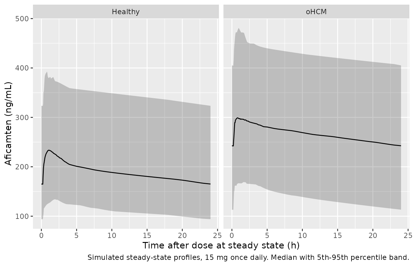
Assumptions and deviations
- Body-weight and sex distributions are assumed. Xu 2025 Table S5 reports only medians, ranges, and sex percentages. Weight is drawn log-normally with the published median and truncated to the published range, using a log-scale SD chosen so the published extremes sit near the tails of a cohort of the published size (SD 0.14 for healthy participants, 0.21 for participants with oHCM). Sex is Bernoulli at the published female percentage. The simulated oHCM AUCtau %CV is consequently somewhat lower than the published 40.3%, because the real cohort’s weight range (47-156 kg) is wider than a truncated log-normal with this SD produces at n = 200.
-
Some Figure 4 reference values are digitised, not
tabulated. Xu 2025 reports Figure 4 only as a graphic. Three of
the six scenario rows and the base-case Ctau were read off the panels;
see the provenance note above the Figure 4 chunk for which values these
are and for the two independent checks that corroborate them. No
digitised value informs any
ini()parameter – they are used solely as validation targets. - Race, age, renal function, and concomitant medications are not simulated. None was retained in the final model (Xu 2025 Section 3.1.2), so they cannot affect predictions.
-
Steady state is imposed exactly rather than approached by a
dose train. Dose records carry
ss = 1withii = 24, so rxode2 places each subject at its analytic steady state. Simulating a finite train of daily doses instead would bias the cohort: the published 308% CV on Vc/F produces a tail of subjects with terminal half-lives beyond 700 h, and after 40 daily doses the worst of them is still 40% short of its steady-state AUCtau. That is not a modelling artifact – it is the paper’s own finding that a protracted right tail in total volume leaves ~5% of participants with oHCM still accumulating at day 33 (Xu 2025 Table 2, Section 3.2.1, Figure 3). Imposing steady state analytically is what lets the structural check below assert theAUCtau = Dose / (CL/F)identity per subject rather than on a cohort median. - Post-hoc Empirical Bayes estimates versus fresh IIV draws. Xu 2025 simulated Table 2 and Figure 4 using each participant’s post-hoc EBEs. This vignette draws fresh random effects from the reported OMEGA. Reported eta-shrinkage was low for CL/F (6.9%), so the AUCtau distribution should be comparable; shrinkage was higher for Vc/F (22.6%) and Vp/F (28.7%), so the simulated spread of Cmax and of the terminal half-life is expected to exceed the published spread somewhat.
-
IIV on Q/F is omitted. The source control stream
fixes it to zero (
$OMEGA 0 FIX ; BSVQ/F) and Table 1 reports no omega for Q/F. Encoding a zero-variance eta would make OMEGA singular and break the Cholesky sampler, so the eta is simply absent. - Half-life is derived two ways. The Figure 3 table computes the analytic terminal (beta) half-life from each subject’s individual CL/F, Vc/F, Q/F, and Vp/F; the NCA comparison estimates it by regression on a simulated single-dose profile truncated at the 1 ng/mL LLOQ. Xu 2025 does not state which route produced its Table 2 values.
Errata
Two numeric conflicts and one internal inconsistency were found in the source. None was resolved by adjusting a parameter.
- Ka: Table 1 reports 0.337 1/h; Figure S3 reports 0.373 1/h. The model uses Table 1’s 0.337. Table 1 is the article’s primary parameter table and reports Ka with a relative standard error (5.03%) taken from the NONMEM covariance step, so it is the artifact read directly off the model output; Figure S3 is a hand-set summary equation that transcribes the same estimates. Figure S3 independently mis-transcribes a second value on the same display (it prints the high-fat-meal effect on F1 as 0.0686 where Table 1 reports 0.0687), which is direct evidence that Figure S3 is the lower-fidelity artifact. The choice is also immaterial to every quantity the paper reports reproducibly: substituting 0.373 changes simulated steady-state AUCtau and Ctau by less than 0.3%, because at a terminal half-life of roughly 80 h the steady-state profile is nearly flat and essentially independent of the absorption rate.
- The high-fat-meal effect on F1 is 0.0687 in Table 1 and 0.0686 in Figure S3. Table 1 is used, for the same reason. The difference is below the resolution of any published check (both give a 6.9% increase in AUCtau, which is what Figure 4 panel A reports).
- The published Cmax column is not reproducible and is internally inconsistent. AUCtau and Ctau reproduce across all six Figure 4 scenarios to within 0.5 percentage points, and the base case reproduces to within 0.5% for AUCtau (5725 versus 5720) and 0.2% for Ctau. The base-case Cmax does not (simulated ~281 versus published 241 ng/mL), and the Cmax percent changes differ from the published ones for the sex and food scenarios. The high-fat-meal row falsifies the published Cmax column on the paper’s own parameters: a high-fat meal reduces Ka by 36.5% and lengthens Tlag by 11.5% while raising F1 by only 6.87%, so it must raise Cmax by less than it raises AUCtau. Solving the steady-state two-compartment profile analytically at the published estimates, the slower absorption almost exactly cancels the bioavailability gain and Cmax moves by under a tenth of a percent (the simulated column above), while AUCtau rises the full 6.9% and Ctau rises 8.4% – both of which the published figure reproduces. Figure 4 nonetheless reports Cmax +12.9%, which no first-order absorption model with a slower Ka can produce. The most likely explanation is that the published Cmax values were read off a discrete nominal sampling grid or computed by a different post-processing route than AUCtau and Ctau; the paper does not state the simulation grid. Parameters were not tuned to close the gap, and the vignette’s assertions deliberately gate AUCtau and Ctau only.
-
Table 1 lists the unit of Ka as “L/h”. Ka is a
first-order rate constant; the Data S1 control stream comments it as
;5 KA 1/hr. The model file uses 1/h. Table S4 carries the same typographical error for the base model. - No erratum or corrigendum was located for this article as of the extraction date.