Prednisolone (Bouazza 2025)
Source:vignettes/articles/Bouazza_2025_prednisolone.Rmd
Bouazza_2025_prednisolone.RmdModel and source
- Citation: Bouazza N, Semeraro M, Lui G, Froelicher-Bournaud L, Choupeaux L, Treluyer JM, Benaboud S, Terzic J, Hachulla E, Remy P, Harambat J, Karras A, Rousset-Rouviere C, Jolivot A, Amoura Z, Daugas E, Hummel A, Salomon R, Lega JC, Decramer S, Belot A, Gobert D, Costedoat-Chalumeau N, Faguer S, Melki I, Jourde-Chiche N, Bader-Meunier B. Population pharmacokinetic modelling of prednisolone in systemic lupus erythematosus patients: Analysis of exposure and disease activity. Br J Clin Pharmacol. 2025;91(10):2854-2864. doi:10.1002/bcp.70103. Protein-binding constants (Bmax, K1, Kns) fixed from Petersen HH, Andreassen TK, Breiderhoff T, et al., as cited by Bouazza 2025 Methods section 2.3 (reference 14).
- Description: One-compartment population PK model for prednisolone (the active metabolite of orally administered prednisone) in 66 paediatric and adult patients with active systemic lupus erythematosus (Bouazza 2025). First-order absorption with a lag time that represents the combined absorption and prednisone-to-prednisolone conversion delay. The disposition is parameterised on UNBOUND prednisolone (CLu/F and Vu/F, allometrically scaled to body weight with fixed exponents 0.75 and 1), which linearises the kinetics; the observed TOTAL plasma concentration is then recovered algebraically through a saturable corticosteroid- binding-globulin plus linear albumin binding model with constants fixed from Petersen 1983. Bioavailability decreases as a power function of the administered prednisone dose.
- Article: https://doi.org/10.1002/bcp.70103
Bouazza and colleagues developed a population pharmacokinetic model for prednisolone, the active metabolite of orally administered prednisone, in patients with active systemic lupus erythematosus (SLE). The model has two features that distinguish it from a routine one-compartment oral popPK model:
-
The disposition is parameterised on unbound drug.
Prednisolone binds saturably to corticosteroid-binding globulin (CBG,
high affinity / low capacity) and linearly to albumin (low affinity /
high capacity). Total prednisolone therefore has markedly non-linear
kinetics, while unbound prednisolone does not. The authors fit
CLu/FandVu/Fon the unbound scale and recover the measured total concentration algebraically. -
Bioavailability falls as the dose rises. A power
function of the administered prednisone dose was added to
F, which is the paper’s central clinical message: raising the prednisone dose beyond a certain point does not raise effective prednisolone exposure proportionally.
Population
The analysis pooled 66 patients with active SLE (34 juvenile-onset, 32 adult-onset) enrolled prospectively at 28 French paediatric and adult university-hospital centres between April 2018 and January 2022 (NCT03187743). Median age was 23 years (IQR 14.2-31.2, range 6-63) and median body weight 56.1 kg (IQR 46.8-66.5, range 17.3-113.5); 80.3% were female. The cohort was ethnically diverse (29.2% Caucasian, 20.0% Asian, 18.5% Sub-Saharan African, 15.4% North African, 10.8% Caribbean, remainder Turkish, Central/South American or mixed). Renal involvement was the most common flare manifestation (74.2%). Concomitant therapy included hydroxychloroquine (87.9%), methylprednisolone boluses (57.6%) and mycophenolate mofetil (53.0%).
Prednisone was given orally at at least 0.5 mg/kg/day at initiation (median 0.94 mg/kg/day, IQR 0.65-1.06, range 0.38-2.3). Sampling was opportunistic during routine care: 242 concentrations, median 3 per patient (range 1-11), drawn 5 min to 32 h after the last dose (median 3.3 h). Thirty-five samples (14%) were below the limit of quantification and were treated as left-censored. Baseline characteristics are from Table 1 of the source.
The same information is available programmatically via the model’s
population metadata
(readModelDb("Bouazza_2025_prednisolone")()$population).
Source trace
The per-parameter origin is recorded as an in-file comment next to
each ini() entry in
inst/modeldb/specificDrugs/Bouazza_2025_prednisolone.R. The
table below collects them in one place for review.
| Equation / parameter | Value | Source location |
|---|---|---|
ltlag (Tlag) |
0.17 h | Table 2, T lag (h), 2% rse |
lka (ka) |
1.19 1/h | Table 2, k a (h-1), 1% rse |
lcl (CLu/F) |
54.3 L/h per 70 kg | Table 2, CL U /F, 7% rse; 95% CI 48-62 (Abstract) |
lvc (Vu/F) |
235 L per 70 kg | Table 2, V U /F, 8% rse; 95% CI 203-274 (Abstract) |
e_wt_cl |
0.75 (fixed) | Table 2 covariate column (BW/70)^0.75; Methods 2.3
“power exponents fixed to 0.75 and 1 for CL and V” |
e_wt_vc |
1 (fixed) | Table 2 covariate column (BW/70)^1; Methods 2.3 |
e_dose_fdepot (betaFdose) |
-0.28 | Table 2, beta Fdose, 2% rse |
| F reference dose | 80 000 nmol | Table 2 covariate column (Dose/80000)^betaFdose;
footnote “80 000 nmol corresponds to 30 mg of prednisone” |
lbmax (Bmax) |
6.77 (fixed) | Table 2, B max, marked * = fixed; Methods
2.3, set per Petersen et al. |
kaff (K1) |
0.0095 L/nmol (fixed) | Table 2, K 1 (L/nmol), marked *
|
kns (Kns) |
0.8 (fixed) | Table 2, K ns, marked *
|
etalcl |
omega 0.35 -> variance 0.1225 | Table 2, omega CL,U, 17% rse |
etalbmax |
omega 0.3 (fixed) -> variance 0.09 | Table 2, omega Bmx, marked *
|
propSd |
0.42 | Table 2, Residual variability, proportional, 7%
rse |
Binding equation
Ctot = Cu * (1 + Bmax/(1 + K1*Cu) + Kns)
|
n/a | Methods 2.3, displayed equation |
Allometric covariate form (BW/70)^exp
|
n/a | Methods 2.3 and Table 2 covariate column |
| One-compartment, first-order absorption with lag | n/a | Results 3.2 first paragraph; Abstract “one-compartment open model with absorption lag time” |
Scale conventions applied during transcription
Two conversions were required and are the most likely places for a transcription error, so they are stated explicitly:
-
Monolix omega is a standard deviation; nlmixr2
ini()takes a variance. Table 2’somega CL,U = 0.35andomega Bmx = 0.3are therefore encoded as0.35^2 = 0.1225and0.3^2 = 0.09. On the SD scale the CL random effect corresponds to a coefficient of variation ofsqrt(exp(0.1225) - 1) = 36.1%. -
The sign of
betaFdose. The published PDF’s minus glyphs are lost in text extraction (the same file renders “-80 degrees C” as “80 C” and “h^-1” as “h1”), so Table 2’sbeta Fdosereads as a bare0.28. The exponent is negative. Three independent lines of evidence fix the sign, and the third is quantitative:
# The Discussion states: for a typical 80 kg patient given 63.5 mg of
# prednisone, the model predicts an apparent unbound clearance of 75 L/h.
# Only the negative exponent reproduces that number.
mw_prednisone <- 358.43            # g/mol
dose_nmol     <- 63.5e-3 / mw_prednisone * 1e9
clu_80kg      <- 54.3 * (80 / 70)^0.75

tibble::tibble(betaFdose = c(-0.28, 0.28)) |>
  dplyr::mutate(
    F_bioav        = (dose_nmol / 80000)^betaFdose,
    apparent_CLu_F = clu_80kg / F_bioav
  ) |>
  knitr::kable(digits = 3,
caption = "Only betaFdose = -0.28 reproduces the Discussion's 75 L/h.")| betaFdose | F_bioav | apparent_CLu_F |
|---|---|---|
| -0.28 | 0.800 | 74.985 |
| 0.28 | 1.249 | 48.041 |
The other two are qualitative and agree: the Abstract states “the bioavailability parameter was found to decrease non-linearly with the dose”, and the What this study adds box states “prednisolone bioavailability appears to decrease as prednisone doses increase”.
Virtual cohort
Original observed data are not publicly available. The simulations below use virtual populations whose covariate distributions approximate the published trial demographics (Table 1).
set.seed(20250818)

mw_prednisone <- 358.43            # g/mol, for mg -> nmol of the dosed prodrug
mg_to_nmol    <- function(mg) mg * 1e6 / mw_prednisone

# Helper: one arm as a self-contained event table. `id_offset` keeps subject
# IDs disjoint so several arms can be bind_rows()-ed safely.
make_cohort <- function(wt, dose_mg, label, obs_times, id_offset = 0L) {
  n <- length(wt)
  subj <- tibble::tibble(
    id        = id_offset + seq_len(n),
    WT        = wt,
    treatment = label,
    dose_nmol = mg_to_nmol(dose_mg)
  )

  doses <- subj |>
    dplyr::mutate(time = 0, amt = dose_nmol, evid = 1L, cmt = "depot")

  # Observation rows point at the ODE state `central`, never at the algebraic
  # observables `Cc` / `Cu` (that would auto-inject a cmt() slot and renumber
  # the compartments).
  obs <- subj |>
    tidyr::crossing(time = obs_times) |>
    dplyr::mutate(amt = NA_real_, evid = 0L, cmt = "central")

  dplyr::bind_rows(doses, obs) |>
    dplyr::arrange(id, time, dplyr::desc(evid))
}

obs_grid <- sort(unique(c(seq(0, 4, by = 0.05), seq(4, 24, by = 0.25))))

# Arm 1 -- the Garg & Jusko replication scenario used in the Discussion:
# a typical 80 kg patient given 63.5 mg of prednisone.
ev_gj <- make_cohort(wt = 80, dose_mg = 63.5, label = "80 kg, 63.5 mg",
                     obs_times = obs_grid, id_offset = 0L)

# Arm 2 -- typical-value dose escalation at a fixed 70 kg body weight, to
# expose the dose-dependent bioavailability.
dose_levels <- c(5, 10, 30, 60, 90, 120)
ev_dose <- dplyr::bind_rows(
  lapply(seq_along(dose_levels), function(i) {
    make_cohort(wt = 70, dose_mg = dose_levels[i],
                label = sprintf("%g mg", dose_levels[i]),
                obs_times = obs_grid, id_offset = 100L * i)
  })
)

# Arm 3 -- a 200-subject cohort matching the Table 1 weight distribution,
# dosed at the cohort median 0.94 mg/kg, for a VPC-style summary.
n_vpc  <- 200
wt_vpc <- pmin(pmax(stats::rlnorm(n_vpc, meanlog = log(56.1), sdlog = 0.2605),
                    17.3), 113.5)
ev_vpc <- make_cohort(wt = wt_vpc, dose_mg = 0.94 * wt_vpc,
                      label = "0.94 mg/kg", obs_times = obs_grid,
                      id_offset = 10000L)

# Regression guard: no duplicated (id, time, evid) triples. Note this must NOT
# be wrapped in unique() -- unique() would remove the very duplicates the
# assertion is meant to detect, making it impossible to fail.
for (ev in list(ev_gj, ev_dose, ev_vpc)) {
  stopifnot(!anyDuplicated(ev[, c("id", "time", "evid")]))
}
stopifnot(length(intersect(ev_dose$id, ev_vpc$id)) == 0)
The weight distribution is a log-normal truncated to the published
range; its sdlog is chosen so the simulated interquartile
range reproduces Table 1’s 46.8-66.5 kg.
tibble::tibble(
  statistic = c("median", "Q1", "Q3", "min", "max"),
  simulated = c(median(wt_vpc), quantile(wt_vpc, 0.25), quantile(wt_vpc, 0.75),
                min(wt_vpc), max(wt_vpc)),
  published = c(56.1, 46.8, 66.5, 17.3, 113.5)
) |>
knitr::kable(digits = 1, caption = "Simulated vs. published body weight (Table 1).")| statistic | simulated | published |
|---|---|---|
| median | 57.8 | 56.1 |
| Q1 | 47.1 | 46.8 |
| Q3 | 66.8 | 66.5 |
| min | 30.4 | 17.3 |
| max | 113.5 | 113.5 |
Simulation
mod         <- readModelDb("Bouazza_2025_prednisolone")
mod_typical <- rxode2::zeroRe(mod)
#> ℹ parameter labels from comments will be replaced by 'label()'

# rxSolve omits the `id` column entirely when the event table holds a single
# subject, which silently breaks every downstream group-by and PKNCA formula.
# Restore it rather than assuming it is present.
solve_keep <- function(model, events) {
  out <- as.data.frame(rxode2::rxSolve(model, events = events,
                                       keep = c("WT", "treatment")))
  if (is.null(out$id)) out$id <- 1L
  out$id <- as.integer(as.character(out$id))
  out
}

sim_gj   <- solve_keep(mod_typical, ev_gj)
#> ℹ omega/sigma items treated as zero: 'etalcl', 'etalbmax'
sim_dose <- solve_keep(mod_typical, ev_dose)
#> ℹ omega/sigma items treated as zero: 'etalcl', 'etalbmax'
#> Warning: multi-subject simulation without without 'omega'
sim_vpc  <- solve_keep(mod, ev_vpc)
#> ℹ parameter labels from comments will be replaced by 'label()'

stopifnot(nrow(sim_gj) > 0, nrow(sim_dose) > 0, nrow(sim_vpc) > 0)
stopifnot(!anyNA(sim_gj$Cc), !anyNA(sim_dose$Cc), !anyNA(sim_vpc$Cc))
stopifnot(all(sim_vpc$Cc >= 0), all(sim_vpc$Cu >= 0))
Both the unbound concentration Cu and the observed total
concentration Cc are returned as columns, because rxode2
evaluates every algebraic observable at each observation record
regardless of which compartment the record points at.
The protein-binding model
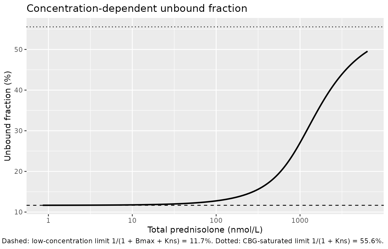
The measured quantity is total plasma prednisolone; the model’s state is unbound. The two are linked by the saturable-plus-linear binding equation of Methods 2.3, with all three constants fixed from Petersen et al.:
At low concentrations CBG is far from saturated and the unbound
fraction is 1 / (1 + 6.77 + 0.8) = 11.7%. As CBG saturates,
the unbound fraction rises towards the albumin-only limit
1 / (1 + 0.8) = 55.6%, which is what makes total
prednisolone kinetics non-linear.
bmax <- 6.77; kaff <- 0.0095; kns <- 0.8

binding <- tibble::tibble(Cu = 10^seq(-1, 3.5, length.out = 400)) |>
  dplyr::mutate(
    Ctot = Cu * (1 + bmax / (1 + kaff * Cu) + kns),
    fu   = Cu / Ctot
  )

# Limiting unbound fractions, checked against the closed forms.
stopifnot(abs(min(binding$fu) - 1 / (1 + bmax + kns)) < 1e-3)
stopifnot(max(binding$fu) < 1 / (1 + kns))

ggplot(binding, aes(Ctot, 100 * fu)) +
  geom_line(linewidth = 0.9) +
  geom_hline(yintercept = 100 / (1 + bmax + kns), linetype = "dashed") +
  geom_hline(yintercept = 100 / (1 + kns), linetype = "dotted") +
  scale_x_log10() +
  labs(
    x = "Total prednisolone (nmol/L)", y = "Unbound fraction (%)",
    title = "Concentration-dependent unbound fraction",
    caption = paste(
      "Encodes the binding equation of Methods 2.3.",
      "Dashed: low-concentration limit 1/(1 + Bmax + Kns) = 11.7%.",
      "Dotted: CBG-saturated limit 1/(1 + Kns) = 55.6%."
    )
  )
Dose-dependent bioavailability
This reproduces the paper’s central clinical claim. Because
F = (Dose/80000)^-0.28, exposure rises less than
proportionally with dose.
auc_trapezoid <- function(time, conc) sum(diff(time) * (head(conc, -1) + tail(conc, -1)) / 2)

dose_summary <- sim_dose |>
  dplyr::group_by(treatment) |>
  dplyr::summarise(
    dose_mg  = unique(as.numeric(sub(" mg", "", treatment))),
    Cmax     = max(Cc),
    AUC24_u  = auc_trapezoid(time, Cu),
    .groups  = "drop"
  ) |>
  dplyr::arrange(dose_mg) |>
  dplyr::mutate(
    F_bioav          = (mg_to_nmol(dose_mg) / 80000)^-0.28,
    AUC_per_mg       = AUC24_u / dose_mg,
    AUC_rel_to_5mg   = AUC24_u / AUC24_u[1],
    dose_rel_to_5mg  = dose_mg / dose_mg[1]
  )

dose_summary |>
  dplyr::select(treatment, F_bioav, Cmax, AUC24_u, AUC_per_mg,
                dose_rel_to_5mg, AUC_rel_to_5mg) |>
  dplyr::rename(
    "Dose"                        = treatment,
    "F"                           = F_bioav,
    "Cmax total (nmol/L)"         = Cmax,
    "AUC0-24 unbound (nmol*h/L)"  = AUC24_u,
    "AUC per mg"                  = AUC_per_mg,
    "Dose ratio vs 5 mg"          = dose_rel_to_5mg,
    "AUC ratio vs 5 mg"           = AUC_rel_to_5mg
  ) |>
  knitr::kable(digits = c(0, 3, 1, 1, 2, 1, 1),
caption = "Dose-dependent bioavailability: a 24-fold dose increase gives a less-than-24-fold exposure increase.")| Dose | F | Cmax total (nmol/L) | AUC0-24 unbound (nmol*h/L) | AUC per mg | Dose ratio vs 5 mg | AUC ratio vs 5 mg |
|---|---|---|---|---|---|---|
| 5 mg | 1.631 | 390.0 | 416.9 | 83.38 | 1 | 1.0 |
| 10 mg | 1.343 | 553.3 | 686.7 | 68.67 | 2 | 1.6 |
| 30 mg | 0.987 | 919.9 | 1514.6 | 50.49 | 6 | 3.6 |
| 60 mg | 0.813 | 1263.7 | 2494.8 | 41.58 | 12 | 6.0 |
| 90 mg | 0.726 | 1533.8 | 3340.5 | 37.12 | 18 | 8.0 |
| 120 mg | 0.670 | 1769.4 | 4109.3 | 34.24 | 24 | 9.9 |
# The exposure ratio must fall below the dose ratio at every level above the
# reference, and AUC per mg must decrease monotonically.
stopifnot(all(dose_summary$AUC_rel_to_5mg[-1] < dose_summary$dose_rel_to_5mg[-1]))
stopifnot(all(diff(dose_summary$AUC_per_mg) < 0))
sim_dose |>
  dplyr::mutate(dose_lbl = factor(treatment,
                                  levels = sprintf("%g mg", sort(dose_levels)))) |>
  ggplot(aes(time, Cc, colour = dose_lbl)) +
  geom_line(linewidth = 0.8) +
  scale_y_log10() +
  labs(x = "Time (h)", y = "Total prednisolone (nmol/L)", colour = "Prednisone dose",
       title = "Typical-value total prednisolone profiles, 70 kg",
       caption = "Dose-dependent F and saturable CBG binding both act here.")
#> Warning in scale_y_log10(): log-10 transformation introduced infinite values.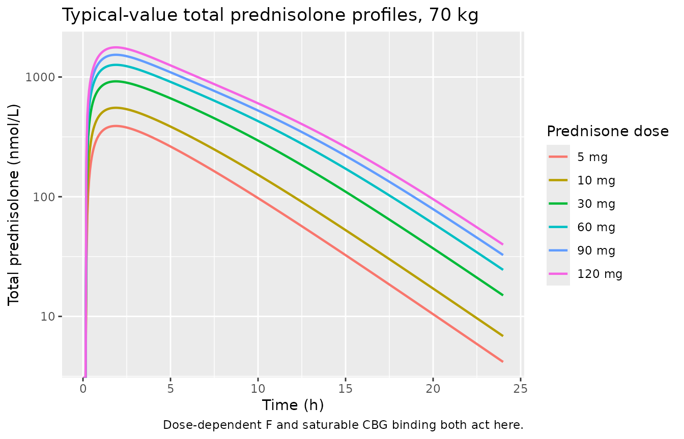
PKNCA validation
The paper reports no NCA table, so the validation targets are the
quantitative statements the authors make about the model itself. PKNCA
is run on both outputs: the unbound profile (the scale on which
CLu/F is defined) and the observed total profile.
nca_conc <- function(sim) {
  out <- sim |>
    dplyr::filter(!is.na(Cc)) |>
    dplyr::select(id, time, Cc, Cu, treatment)
  # Guarantee a time-zero record so PKNCA can anchor AUC from 0. Pre-dose
  # concentration is 0 for this extravascular model.
  dplyr::bind_rows(
    out,
    out |> dplyr::distinct(id, treatment) |> dplyr::mutate(time = 0, Cc = 0, Cu = 0)
  ) |>
    dplyr::distinct(id, treatment, time, .keep_all = TRUE) |>
    dplyr::arrange(id, treatment, time)
}

nca_dose <- function(ev) {
  ev |> dplyr::filter(evid == 1) |> dplyr::select(id, time, amt, treatment)
}

gj_conc <- nca_conc(sim_gj)

# Unbound: CLu/F = Dose / AUCinf on the unbound scale.
conc_u <- PKNCA::PKNCAconc(gj_conc, Cu ~ time | treatment + id,
                           concu = "nmol/L", timeu = "h")
dose_u <- PKNCA::PKNCAdose(nca_dose(ev_gj), amt ~ time | treatment + id,
                           doseu = "nmol")

intervals_u <- data.frame(start = 0, end = Inf,
                          cmax = TRUE, tmax = TRUE, aucinf.obs = TRUE,
                          half.life = TRUE, cl.obs = TRUE)

nca_u <- PKNCA::pk.nca(PKNCA::PKNCAdata(conc_u, dose_u, intervals = intervals_u))
nca_u_tbl <- as.data.frame(nca_u$result)
knitr::kable(nca_u_tbl, digits = 3,
caption = "PKNCA on the unbound profile, 80 kg / 63.5 mg prednisone.")| treatment | id | start | end | PPTESTCD | PPORRES | exclude | PPORRESU |
|---|---|---|---|---|---|---|---|
| 80 kg, 63.5 mg | 1 | 0 | Inf | cmax | 358.670 | NA | nmol/L |
| 80 kg, 63.5 mg | 1 | 0 | Inf | tmax | 1.900 | NA | h |
| 80 kg, 63.5 mg | 1 | 0 | Inf | tlast | 24.000 | NA | h |
| 80 kg, 63.5 mg | 1 | 0 | Inf | clast.obs | 3.163 | NA | nmol/L |
| 80 kg, 63.5 mg | 1 | 0 | Inf | lambda.z | 0.221 | NA | 1/h |
| 80 kg, 63.5 mg | 1 | 0 | Inf | r.squared | 1.000 | NA | unitless |
| 80 kg, 63.5 mg | 1 | 0 | Inf | adj.r.squared | 1.000 | NA | unitless |
| 80 kg, 63.5 mg | 1 | 0 | Inf | lambda.z.time.first | 2.900 | NA | h |
| 80 kg, 63.5 mg | 1 | 0 | Inf | lambda.z.time.last | 24.000 | NA | h |
| 80 kg, 63.5 mg | 1 | 0 | Inf | lambda.z.n.points | 103.000 | NA | count |
| 80 kg, 63.5 mg | 1 | 0 | Inf | clast.pred | 3.206 | NA | nmol/L |
| 80 kg, 63.5 mg | 1 | 0 | Inf | half.life | 3.129 | NA | h |
| 80 kg, 63.5 mg | 1 | 0 | Inf | span.ratio | 6.742 | NA | fraction |
| 80 kg, 63.5 mg | 1 | 0 | Inf | aucinf.obs | 2362.781 | NA | h*nmol/L |
| 80 kg, 63.5 mg | 1 | 0 | Inf | cl.obs | 74.980 | NA | nmol/(h*nmol/L) |
conc_t <- PKNCA::PKNCAconc(gj_conc, Cc ~ time | treatment + id,
                           concu = "nmol/L", timeu = "h")
dose_t <- PKNCA::PKNCAdose(nca_dose(ev_gj), amt ~ time | treatment + id,
                           doseu = "nmol")

nca_t <- PKNCA::pk.nca(PKNCA::PKNCAdata(conc_t, dose_t, intervals = intervals_u))
nca_t_tbl <- as.data.frame(nca_t$result)
knitr::kable(nca_t_tbl, digits = 3,
caption = "PKNCA on the observed total profile, same subject.")| treatment | id | start | end | PPTESTCD | PPORRES | exclude | PPORRESU |
|---|---|---|---|---|---|---|---|
| 80 kg, 63.5 mg | 1 | 0 | Inf | cmax | 1196.546 | NA | nmol/L |
| 80 kg, 63.5 mg | 1 | 0 | Inf | tmax | 1.900 | NA | h |
| 80 kg, 63.5 mg | 1 | 0 | Inf | tlast | 24.000 | NA | h |
| 80 kg, 63.5 mg | 1 | 0 | Inf | clast.obs | 26.485 | NA | nmol/L |
| 80 kg, 63.5 mg | 1 | 0 | Inf | lambda.z | 0.213 | NA | 1/h |
| 80 kg, 63.5 mg | 1 | 0 | Inf | r.squared | 1.000 | NA | unitless |
| 80 kg, 63.5 mg | 1 | 0 | Inf | adj.r.squared | 1.000 | NA | unitless |
| 80 kg, 63.5 mg | 1 | 0 | Inf | lambda.z.time.first | 17.250 | NA | h |
| 80 kg, 63.5 mg | 1 | 0 | Inf | lambda.z.time.last | 24.000 | NA | h |
| 80 kg, 63.5 mg | 1 | 0 | Inf | lambda.z.n.points | 28.000 | NA | count |
| 80 kg, 63.5 mg | 1 | 0 | Inf | clast.pred | 26.677 | NA | nmol/L |
| 80 kg, 63.5 mg | 1 | 0 | Inf | half.life | 3.262 | NA | h |
| 80 kg, 63.5 mg | 1 | 0 | Inf | span.ratio | 2.069 | NA | fraction |
| 80 kg, 63.5 mg | 1 | 0 | Inf | aucinf.obs | 10320.786 | NA | h*nmol/L |
| 80 kg, 63.5 mg | 1 | 0 | Inf | cl.obs | 17.166 | NA | nmol/(h*nmol/L) |
Comparison against the published values
getp <- function(tbl, code) {
  v <- tbl$PPORRES[tbl$PPTESTCD == code]
  if (length(v) != 1L) stop("no unique PKNCA row for '", code, "'")
  v
}

clu_f_sim <- getp(nca_u_tbl, "cl.obs")
thalf_sim <- getp(nca_u_tbl, "half.life")

# Closed-form references derived from the published point estimates.
clu_80  <- 54.3 * (80 / 70)^0.75
vu_80   <- 235 * (80 / 70)
F_gj    <- (mg_to_nmol(63.5) / 80000)^-0.28

comparison <- tibble::tribble(
  ~Quantity,                                        ~Reference, ~`Reference source`,                       ~Simulated,
  "Apparent unbound clearance CLu/F (L/h)",          75.0,       "Discussion, model prediction",             clu_f_sim,
  "Apparent unbound clearance CLu/F (L/h)",          86.0,       "Discussion, Garg & Jusko observed",        clu_f_sim,
  "Unbound terminal half-life (h)",                  log(2) * vu_80 / clu_80, "log(2)*Vu/CLu from Table 2",  thalf_sim,
  "Bioavailability F at 63.5 mg",                    F_gj,       "Table 2 (Dose/80000)^-0.28",               clu_80 / clu_f_sim
) |>
  dplyr::mutate(`% diff` = 100 * (Simulated - Reference) / Reference)

comparison |>
  knitr::kable(digits = 2,
caption = "Simulated vs. published / closed-form reference values.")| Quantity | Reference | Reference source | Simulated | % diff |
|---|---|---|---|---|
| Apparent unbound clearance CLu/F (L/h) | 75.0 | Discussion, model prediction | 74.98 | -0.03 |
| Apparent unbound clearance CLu/F (L/h) | 86.0 | Discussion, Garg & Jusko observed | 74.98 | -12.81 |
| Unbound terminal half-life (h) | 3.1 | log(2)*Vu/CLu from Table 2 | 3.13 | 0.90 |
| Bioavailability F at 63.5 mg | 0.8 | Table 2 (Dose/80000)^-0.28 | 0.80 | 0.01 |
The model reproduces the paper’s own stated prediction of 75
L/h for a typical 80 kg patient receiving 63.5 mg of
prednisone. That number is a genuine answer key: it appears in the
Discussion, it is not one of the fitted parameters, and it depends
jointly on the clearance estimate, the allometric exponent, the
dose-to-nmol conversion and the sign and magnitude of
betaFdose. Reproducing it therefore checks the whole chain
at once.
The 86 L/h row is the observed value Garg and Jusko reported in a separate 12-subject study; the authors quote it as external corroboration, and the ~13% gap between it and the model prediction is the authors’ own, not a defect introduced here.
# Gate 1: on the unbound scale the model is linear, so AUCinf must equal
# Dose * F / CLu exactly. This simultaneously checks the dose units, the
# allometric scaling, the F term and the PKNCA setup.
auc_u_sim <- getp(nca_u_tbl, "aucinf.obs")
auc_u_ref <- mg_to_nmol(63.5) * F_gj / clu_80
stopifnot(abs(auc_u_sim - auc_u_ref) / auc_u_ref < 0.005)

# Gate 2: apparent unbound clearance must recover the Discussion's 75 L/h.
stopifnot(abs(clu_f_sim - 75) / 75 < 0.02)

# Gate 3: unbound terminal half-life must equal log(2)*Vu/CLu.
stopifnot(abs(thalf_sim - log(2) * vu_80 / clu_80) / (log(2) * vu_80 / clu_80) < 0.02)

# Gate 4: allometry. Doubling weight must scale CLu by 2^0.75 and Vu by 2.
ev_allo <- dplyr::bind_rows(
  make_cohort(35, 30, "35 kg", obs_grid, id_offset = 50000L),
  make_cohort(70, 30, "70 kg", obs_grid, id_offset = 60000L)
)
sim_allo <- solve_keep(mod_typical, ev_allo)
#> ℹ omega/sigma items treated as zero: 'etalcl', 'etalbmax'
#> Warning: multi-subject simulation without without 'omega'
cl_allo <- sim_allo |>
  dplyr::group_by(treatment) |>
  dplyr::summarise(auc = auc_trapezoid(time, Cu), WT = unique(WT), .groups = "drop") |>
  dplyr::mutate(cl_apparent = mg_to_nmol(30) / auc)
ratio_cl <- cl_allo$cl_apparent[cl_allo$WT == 70] / cl_allo$cl_apparent[cl_allo$WT == 35]
stopifnot(abs(ratio_cl - 2^0.75) / 2^0.75 < 0.02)

cat(sprintf("AUCinf unbound: sim %.1f vs closed form %.1f (%.3f%%)\n",
            auc_u_sim, auc_u_ref, 100 * (auc_u_sim - auc_u_ref) / auc_u_ref))
#> AUCinf unbound: sim 2362.8 vs closed form 2362.6 (0.006%)
cat(sprintf("CLu/F: sim %.2f vs published 75 L/h (%.2f%%)\n",
            clu_f_sim, 100 * (clu_f_sim - 75) / 75))
#> CLu/F: sim 74.98 vs published 75 L/h (-0.03%)
cat(sprintf("Allometric CL ratio 70kg/35kg: %.4f vs 2^0.75 = %.4f\n",
            ratio_cl, 2^0.75))
#> Allometric CL ratio 70kg/35kg: 1.6872 vs 2^0.75 = 1.6818
Population simulation
vpc <- sim_vpc |>
  dplyr::group_by(time) |>
  dplyr::summarise(
    Q05 = quantile(Cc, 0.05), Q50 = quantile(Cc, 0.50), Q95 = quantile(Cc, 0.95),
    .groups = "drop"
  )

ggplot(vpc, aes(time, Q50)) +
  geom_ribbon(aes(ymin = Q05, ymax = Q95), alpha = 0.25) +
  geom_line(linewidth = 0.9) +
  scale_y_log10() +
  labs(x = "Time (h)", y = "Total prednisolone (nmol/L)",
       title = "Simulated total prednisolone, 200 subjects at 0.94 mg/kg prednisone",
       caption = paste("Median and 5th-95th percentiles. Comparable in shape and",
                       "spread to the prediction-corrected VPC of Figure 1."))
#> Warning in scale_y_log10(): log-10 transformation introduced infinite values.
#> log-10 transformation introduced infinite values.
#> log-10 transformation introduced infinite values.
#> log-10 transformation introduced infinite values.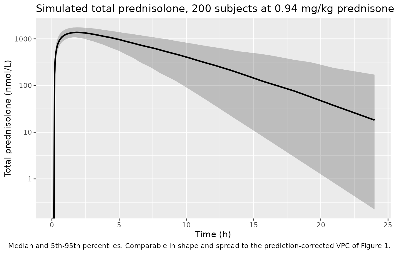
The assay was linear over 5-500 ng/mL, i.e. 13.9-1387 nmol/L for prednisolone (molecular weight 360.44). The simulated median peak sits inside that window, consistent with the observed data in Figure 1.
peak_median <- max(vpc$Q50)
tibble::tibble(
  quantity = c("Simulated median Cmax (nmol/L)",
               "Assay lower limit (nmol/L)",
               "Assay upper limit (nmol/L)"),
  value    = c(peak_median, 5 / 360.44 * 1000, 500 / 360.44 * 1000)
) |>
knitr::kable(digits = 1, caption = "Simulated peak against the published assay range.")| quantity | value |
|---|---|
| Simulated median Cmax (nmol/L) | 1375.0 |
| Assay lower limit (nmol/L) | 13.9 |
| Assay upper limit (nmol/L) | 1387.2 |
Assumptions and deviations
-
Body-weight distribution. Table 1 reports median,
IQR and range but not a distributional family. A log-normal truncated to
the published range is used, with
sdlogchosen to reproduce the published IQR. Age, sex and ethnicity are not model covariates, so they are not simulated. -
Dose units. The model doses in nmol of
prednisone, matching Table 2’s
Dosedefinition and its footnote (“80 000 nmol corresponds to 30 mg of prednisone”). Conversion in this vignette uses the prednisone molecular weight 358.43 g/mol; on that basis 30 mg is 83 697 nmol, so the paper’s “80 000 nmol is about 30 mg” is a rounded statement of the reference dose, and 80 000 nmol is used as the reference exactly as printed. -
betaFdosesign. Encoded as-0.28. The sign is not directly legible in the extracted text because the PDF’s minus glyphs are dropped; it is fixed by the Abstract, the What this study adds box and the quantitative check above. -
Fabove 1 at low doses. BecauseFis fixed to 1 at the 80 000 nmol reference and modified by a negative power, doses below the reference giveF > 1. This is what Table 2 specifies.Fhere is an apparent quantity confounded withCLu/FandVu/F, so a value above 1 is not physically impossible, but simulations far below the studied dose range should be treated with caution: the observed range was at least 0.5 mg/kg/day. -
Prednisone-to-prednisolone conversion. The model
does not carry a separate prednisone compartment. The conversion delay
is absorbed into the lag time (as the Abstract states) and the
conversion extent into
F; the 1:1 molar stoichiometry means the nmol dose carries through unchanged. -
Between-subject variability. Only
CLuandBmaxcarry BSV in the final model. No BSV is reported onTlag,kaorVu, so none is encoded – no variance was invented for them. -
Binding constants are external.
Bmax,K1andKnswere fixed from Petersen et al. rather than estimated in this analysis (Table 2 marks all three with*). They are encoded withfixed()accordingly. - Supplementary material. Supplemental files S1-S4 (covariate correlation plot, Monolix code of the final model, goodness-of-fit plots, BLQ predictive check) are referenced by the paper but could not be obtained when this model was built. Every value used here comes from Table 2 and the Methods text of the main article, which are complete for the final model; the Monolix code in S2 would provide an independent confirmation of the equation forms but is not required to reproduce them.
- Validation targets. The paper reports no NCA table, so the comparison table uses the authors’ own quantitative statement (75 L/h) plus closed-form identities derived from the Table 2 point estimates. No parameter was tuned.