Voriconazole + posaconazole / flucloxacillin drug-drug interaction (Abdullah-Koolmees 2024)
Source:vignettes/articles/AbdullahKoolmees_2024_voriconazole_flucloxacillin_ddi.Rmd
AbdullahKoolmees_2024_voriconazole_flucloxacillin_ddi.RmdModel and source
This paper contributed two model files, one per azole:
-
AbdullahKoolmees_2024_voriconazole_pbpk– the whole-body PBPK model whose saturable CYP metabolism carries the drug-drug interaction. -
AbdullahKoolmees_2024_posaconazole_pbpk– the comparator arm, structurally identical but with linear hepatic clearance and no CYP-mediated interaction.
vori <- readModelDb("AbdullahKoolmees_2024_voriconazole_pbpk")
posa <- readModelDb("AbdullahKoolmees_2024_posaconazole_pbpk")- Citation: Abdullah-Koolmees H, van den Nieuwendijk JF, ten Hoope SMK, de Leeuw DC, Franken LGW, Said MM, Seefat MR, Swart EL, Hendrikse NH, Bartelink IH. Whole Body Physiologically Based Pharmacokinetic Model to Explain A Patient With Drug-Drug Interaction Between Voriconazole and Flucloxacillin. Eur J Drug Metab Pharmacokinet. 2024;49(6):689-699. doi:10.1007/s13318-024-00916-1. Model equations from Electronic Supplementary Material Appendix I equations 8-18 and the accompanying full R/deSolve source listing; drug-specific parameters from Table 1; tissue Kpu, volumes and blood flows from Table 3; CYP Michaelis constants, their flucloxacillin- induced values and the infection-related Vmax fold decreases from Table 5.
- Article: https://doi.org/10.1007/s13318-024-00916-1
- Supplement (Appendix I – all model equations and the full R/deSolve source): https://doi.org/10.1007/s13318-024-00916-1 (Electronic Supplementary Material 1)
Description (voriconazole): PBPK (14-compartment whole-body, perfusion-limited, R/deSolve). Voriconazole disposition in a typical 73-kg adult after oral dosing, built by Abdullah-Koolmees et al. (2024) to explain the clinically observed drug-drug interaction with flucloxacillin. Twelve perfusion-limited tissues plus venous and arterial blood pools are driven by Rodgers-type tissue-to-unbound-plasma partition coefficients (Kpu). Gut and spleen drain into the liver through the portal circulation; the liver is the site of saturable Michaelis-Menten metabolism by CYP2C19, CYP3A4 and CYP2C9 acting on unbound drug, scaled to a whole-organ clearance through the microsomal-protein-per-gram-liver route, and the kidney carries a small linear clearance. Two disease/interaction perturbations are carried as covariates: flucloxacillin co-administration (CONMED_FLUCLOXACILLIN) lowers the CYP Michaelis constants from a user-settable onset time, representing PXR-mediated CYP induction, and an active severe infection (DIS_INFECT_ACTIVE) lowers the CYP Vmax values. Plasma protein binding enters as the fraction-unbound covariate FU, which the source varies between the healthy/DDI and the ICU scenarios. The companion posaconazole model is modellib(‘AbdullahKoolmees_2024_posaconazole_pbpk’).
Description (posaconazole): PBPK (14-compartment whole-body, perfusion-limited, R/deSolve). Posaconazole disposition in a typical 73-kg adult after oral dosing, built by Abdullah-Koolmees et al. (2024) as the comparator arm to their voriconazole model, to test whether flucloxacillin lowers posaconazole exposure the way it lowers voriconazole exposure. The structure, physiology and blood flows are identical to the voriconazole model - twelve perfusion-limited tissues plus venous and arterial blood pools, with gut and spleen draining into the liver - but the drug is far more highly bound (fraction unbound 0.02) and its elimination is linear: posaconazole is 83% excreted unchanged and only minimally metabolised, by UGT1A4 glucuronidation rather than by cytochrome P450, so a single population hepatic clearance replaces the saturable multi-CYP liver model. Because the pregnane X receptor upregulation that flucloxacillin causes acts on CYP enzymes, the authors assumed posaconazole metabolism is unaffected, which the model reproduces as unchanged plasma concentrations across every interaction and inflammation scenario. The companion voriconazole model is modellib(‘AbdullahKoolmees_2024_voriconazole_pbpk’).
Clinical background
A 48-year-old woman with relapsed acute myeloid leukaemia was admitted with Staphylococcus aureus cellulitis and started on intravenous flucloxacillin 6 g daily. She subsequently developed probable pulmonary aspergillosis and was started on oral voriconazole (400 mg twice daily loading over 24 h, then 200 mg twice daily) in the intensive care unit. A trough sample taken after two days of voriconazole was undetectable (< 0.1 mg/L). Voriconazole was replaced by posaconazole 300 mg twice daily; flucloxacillin was continued unchanged, and posaconazole troughs were therapeutic throughout (2.35, 5.21 and 3.35 mg/L, against a > 1.5 mg/L target).
The authors first tested ex vivo whether flucloxacillin displaces voriconazole from albumin. It does not: across five therapeutic-drug-monitoring samples the mean voriconazole free fraction was 40% in control, 44% at a low flucloxacillin concentration (50 mg/L) and 45% at a high concentration (300 mg/L). Having rejected the protein-binding hypothesis, they built the whole-body PBPK model packaged here to test the alternative mechanism: flucloxacillin is a pregnane X receptor (PXR) agonist, and PXR-mediated upregulation of CYP2C19, CYP3A4 and CYP2C9 accelerates voriconazole metabolism.
Population
This is a deterministic single-patient simulation model, not a population fit. The authors state explicitly that no pharmacokinetic variability or covariate variance could be included because of the retrospective single-case design, so exactly one simulation was run per scenario. Accordingly, neither model carries between-subject variability, and the residual-error parameter is fixed at zero rather than invented.
Six typical patients were simulated (source Table 4), differing only in the fraction unbound in plasma and in the two perturbation flags:
scenarios <- tibble::tribble(
  ~scenario, ~label,                        ~FU,  ~CONMED_FLUCLOXACILLIN, ~DIS_INFECT_ACTIVE, ~albumin_g_L, ~crp_mg_L,
  1L, "(1) Case patient: ICU + DDI, low CRP", 0.42, 1, 0, "33-52, median 40", "33 (< 40)",
  2L, "(2) Healthy patient",                  0.42, 0, 0, "33-52, median 40", "< 40",
  3L, "(3) Bacterial infected patient",       0.42, 0, 1, "33-52, median 40", "40-200",
  4L, "(4) DDI with high CRP",                0.42, 1, 1, "33-52, median 40", "40-200",
  5L, "(5) ICU non-infected patient",         0.49, 0, 0, "13.8-38.7, median 30", "< 50",
  6L, "(6) ICU severely infected patient",    0.49, 0, 1, "13.8-38.7, median 30", "> 200"
)
scenarios |>
  dplyr::select(-scenario) |>
  dplyr::rename(
    "Simulated patient" = label,
    "FU"                = FU,
    "Flucloxacillin"    = CONMED_FLUCLOXACILLIN,
    "Active infection"  = DIS_INFECT_ACTIVE,
    "Albumin (g/L)"     = albumin_g_L,
    "CRP (mg/L)"        = crp_mg_L
  ) |>
knitr::kable(caption = "Simulated patient types, reproducing source Table 4.")| Simulated patient | FU | Flucloxacillin | Active infection | Albumin (g/L) | CRP (mg/L) |
|---|---|---|---|---|---|
| (1) Case patient: ICU + DDI, low CRP | 0.42 | 1 | 0 | 33-52, median 40 | 33 (< 40) |
| (2) Healthy patient | 0.42 | 0 | 0 | 33-52, median 40 | < 40 |
| (3) Bacterial infected patient | 0.42 | 0 | 1 | 33-52, median 40 | 40-200 |
| (4) DDI with high CRP | 0.42 | 1 | 1 | 33-52, median 40 | 40-200 |
| (5) ICU non-infected patient | 0.49 | 0 | 0 | 13.8-38.7, median 30 | < 50 |
| (6) ICU severely infected patient | 0.49 | 0 | 1 | 13.8-38.7, median 30 | > 200 |
Model qualification used external literature rather than a fitted dataset: healthy-volunteer plasma profiles from Purkins 2002, steady-state troughs across inflammation stages from van Wanrooy 2014, and post-mortem lung and liver concentrations from eight deceased patients in Weiler 2011 (voriconazole) and five in Blennow 2014 (posaconazole). The acceptance criterion was agreement within 2-fold.
The same information is available programmatically via
readModelDb("AbdullahKoolmees_2024_voriconazole_pbpk")()$population.
Source trace
Every ini() entry in both model files carries an in-file
comment naming its source location. Collected here for review:
| Equation / parameter | Value | Source location |
|---|---|---|
| Tissue Kpu prediction (equations 1-6) | n/a | Appendix I “Tissue drug distribution model”; Rodgers 2005/2006 weak-base model |
Kp = Kpu * Fu (equation 7) |
n/a | Appendix I equation 7 |
| Non-eliminating tissue ODE (equation 8) | n/a | Appendix I equation 8 |
| Lung ODE (equation 9) | n/a | Appendix I equation 9 |
| Venous / arterial ODEs (equations 10-11) | n/a | Appendix I equations 10-11 |
| Gut lumen / gut wall ODEs (equations 12-13) | n/a | Appendix I equations 12-13 |
| Saturable CYP metabolism (equation 15) | n/a | Appendix I equation 15 |
| Hepatic clearance scaling (equation 16) | n/a | Appendix I equation 16 |
| Liver ODE (equation 17) | n/a | Appendix I equation 17 |
| Kidney ODE (equation 18) | n/a | Appendix I equation 18 |
Tissue volumes v_*
|
18.2, 10.5, 1.45, 0.65, 0.33, 0.31, 1.8, 0.5, 29, 0.15, 5.6 L | Table 3 “Tissue volume (L)”; supplement “System Parameters” |
Cardiac output q_co
|
390 L/h | Supplement CA = 6.5 * 60
|
Blood-flow fractions fq_*
|
0.05, 0.05, 0.12, 0.15, 0.04, 0.19, 0.17, 0.03, 0.065 | Supplement Qxx = <fraction> * CA; resulting L/h
in Table 3 |
Blood split f_venous / f_arterial
|
0.705 / 0.295 | Supplement Vve = 0.705*Vbl,
Var = 0.295*Vbl
|
wt_ref |
73 kg | Supplement Weight = 73
|
Voriconazole kpu_* (bone .. rest of body) |
0.62, 0.91, 1.06, 1.03, 1.00, 0.89, 1.08, 0.86, 0.93, 1.03 | Table 3 “Kpu Voriconazole” |
Voriconazole kpu_adipose
|
0.7815 | Appendix I equations 1-4 evaluated with the Table 1
Log Vegetable oil:water (adipose) (Pv) row;
not Table 3, which prints 1.76 – see Errata 12 |
Posaconazole kpu_* (bone .. rest of body) |
5.44, 3.33, 8.73, 8.57, 7.35, 5.07, 11.21, 3.95, 5.64, 7.09 | Table 3 “Kpu Posaconazole” |
Posaconazole kpu_adipose
|
6.5501 | Appendix I equations 1-4 with the Table 1 Pv row;
not Table 3, which prints 7.17 – see Errata 12 |
Voriconazole lka / lfdepot /
bp
|
0.849 /h, 0.96, 1 | Table 1 “Ka”, “F (%)”, “Blood:plasma ratio” |
Posaconazole lka / lfdepot
|
0.795 /h, 0.08 | Supplement KaP, FP; Discussion “worst-case
scenario of only 8% availability” |
vmax_cyp2c19 / cyp3a4 /
cyp2c9
|
40, 32.2, 0.056 pmol/min/pmol | Table 1 “Vmax (pmole/min/pmole)”; supplement
Vmax_2C19/3A4/2C9
|
km_cyp2c19 / cyp3a4 /
cyp2c9
|
9.3, 834.7, 20 uM | Table 1 “Km (um)”; Table 5 “Km value at baseline” |
km_*_ind (flucloxacillin-induced) |
3.72, 181.45, 13.33 uM | Table 5 “Km upregulation (t > 24)” |
tind |
24 h | Supplement if (t < 24) ... else ...; Table 5
header |
finf_cyp2c19 / cyp3a4 /
cyp2c9
|
1.79, 4.6, 1.5 | Table 5 “Decrease in Vmax activity (fold)” |
fumic / mppgl
|
0.711, 30.3 mg/g | Supplement fumic, MPPGL
|
lclr (voriconazole renal) |
0.096 L/h | Supplement CL_ki = 0.096
|
lclpop (posaconazole hepatic) |
8.02 L/h | Table 1 “CL (L/h)”; supplement
Pos_CL_pop = 8.02/FP
|
propSd |
fixed 0 | Not reported – Methods 2.4 single-patient deterministic simulation |
Verification against the published R/deSolve source
The supplement publishes the complete R source of the model, so this extraction can be checked directly rather than only against tabulated outputs. Two independent checks were run while preparing the extraction.
1. The tissue Kpu table is reproducible from the Appendix I equations, and doing so exposes a transcription defect in Table 3. Re-running the Rodgers equations with the supplement’s own tissue-composition constants reproduces nine of the ten Table 3 tissues to within 0.005 absolute for voriconazole (liver 0.895 vs 0.89 published, lung 1.079 vs 1.08, bone 0.617 vs 0.62) and to within 0.13% relative for posaconazole (lung 11.210 vs 11.21, heart 8.571 vs 8.57).
The tenth is adipose, and it does not reproduce.
Appendix I states that the “Vegetable oil:water partition coefficient
(Pv) is used for adipose tissue”; Table 1 tabulates that row explicitly
as Log Vegetable oil:water (adipose) (Pv) – 0.66 for
voriconazole, 4.68 for posaconazole – and the supplement source assigns
it (P_voV <- 1.115 * PV - 1.35 = 0.657). Evaluating the
Appendix I equations that way gives an adipose Kpu of
0.7815 (voriconazole) and 6.5501
(posaconazole). Table 3 instead prints 1.76 and 7.17, which are exactly
what the same equations return if the ordinary octanol logP is
substituted (1.757 and 7.171). Table 3’s adipose row was therefore
produced without the substitution the paper’s own Methods prescribe.
Check 3 below shows which value the authors actually simulated with.
The packaged models use the Pv-derived values.
The rest-of-body Kpu, which the supplement defines as the unweighted mean of all thirteen tissue Kpu values, comes out at 0.939 (voriconazole) and 6.843 (posaconazole) against Table 3’s 1.03 and 7.09 – close, but not an exact reproduction, so the packaged models use the tabulated values there.
2. This rxode2 encoding reproduces the published deSolve
model exactly. A verbatim transcription of the supplement’s
Voriconazole_DDI function, driven with the same dosing and
the same Kpu inputs, was solved with deSolve and compared
against the packaged rxode2 model point-by-point over the final
steady-state dosing interval. The largest relative difference across the
interval is 1.6e-08 – solver noise, not a structural
difference. The mass balance also closes exactly: the ten arterial
branch flows sum to 390.0000 L/h, the cardiac output.
3. The adipose ambiguity is settled by the paper’s own output table. The two candidate adipose Kpu values were run through the verbatim deSolve transcription across all six Table 4 scenarios and scored against the Table 6 predicted plasma concentrations:
| Simulated patient | Table 6 |
Pv adipose (0.7815) |
ratio | Table 3 adipose (1.76) | ratio |
|---|---|---|---|---|---|
| (1) Case patient: ICU + DDI, low CRP | 0.019 | 0.0198 | 1.04 | 0.0518 | 2.73 |
| (2) Healthy patient | 0.431 | 0.4346 | 1.01 | 0.6238 | 1.45 |
| (3) Bacterial infected patient | 0.871 | 1.6629 | 1.91 | 1.9796 | 2.27 |
| (4) DDI with high CRP | 0.235 | 0.1821 | 0.77 | 0.3059 | 1.30 |
| (5) ICU non-infected patient | 0.360 | 0.3693 | 1.03 | 0.5355 | 1.49 |
| (6) ICU severely infected patient | 1.707 | 1.4242 | 0.83 | 1.7030 | 1.00 |
The Pv value puts all six scenarios inside the paper’s
own 2-fold acceptance criterion (geometric mean absolute fold error
1.21) where Table 3’s value puts only four inside it (1.61). More
tellingly, scenarios 1, 2 and 5 – the three that carry
no infection Vmax adjustment and therefore test the
structure and the Km switch alone – are reproduced to within 4% by the
Pv value and are off by 45% to 173% with Table 3’s. The
packaged models use the Pv-derived values; Table 3’s
adipose row is treated as a transcription defect.
4. The infection Vmax effect is part of the model the authors
ran, even though the printed code omits it. Repeating the scan
with DIS_INFECT_ACTIVE forced to 0 everywhere collapses
agreement for the three infected scenarios – ratios fall to 0.50
(scenario 3), 0.08 (scenario 4) and 0.22 (scenario 6), and the geometric
mean absolute fold error rises from 1.21 to 2.22. The Table 5 “Decrease
in Vmax activity (fold)” column is therefore load-bearing for Table 6,
and the published code listing is an incomplete excerpt rather than the
whole model.
Simulation
Both models expose the scenario as data columns, so all six published
patient types are driven from one event table. Note the compartment
names used on observation rows: venous is the ODE state,
and Cc, Clung and Cliver come
back automatically as algebraic observables.
# One deterministic subject per scenario; disjoint ids.
tau  <- 12                 # dosing interval (h)
tend <- 600                # simulate to steady state (h)

make_arm <- function(row) {
  dose_times <- c(0, 12, seq(24, tend - tau, by = tau))
  dose_amt   <- c(400, 400, rep(200, length(dose_times) - 2))
  dplyr::bind_rows(
    tibble::tibble(id = row$scenario, time = dose_times, amt = dose_amt,
                   evid = 1L, cmt = "depot"),
    tibble::tibble(id = row$scenario, time = seq(0, tend, by = 0.25),
                   amt = NA_real_, evid = 0L, cmt = "venous")
  ) |>
    dplyr::mutate(
      label                 = row$label,
      FU                    = row$FU,
      CONMED_FLUCLOXACILLIN = row$CONMED_FLUCLOXACILLIN,
      DIS_INFECT_ACTIVE     = row$DIS_INFECT_ACTIVE
    ) |>
    dplyr::arrange(time, dplyr::desc(evid))
}

events_vori <- dplyr::bind_rows(
  lapply(seq_len(nrow(scenarios)), function(i) make_arm(scenarios[i, ]))
)
stopifnot(!anyDuplicated(unique(events_vori[, c("id", "time", "evid")])))
sim_vori <- rxode2::rxSolve(
  vori, events = events_vori,
  keep = c("label", "FU", "CONMED_FLUCLOXACILLIN", "DIS_INFECT_ACTIVE"),
  atol = 1e-10, rtol = 1e-8
) |>
  as.data.frame() |>
  dplyr::mutate(label = as.character(label))
#> Warning: multi-subject simulation without without 'omega'

nrow(sim_vori)
#> [1] 14406
range(sim_vori$Cc, na.rm = TRUE)
#> [1]  0.00000 11.39281
Replicate published figures
Figure 3A – voriconazole plasma concentration at steady state
# Replicates Figure 3A of Abdullah-Koolmees 2024: voriconazole plasma
# concentration-time profile over one steady-state dosing interval, by
# simulated patient type. Dotted lines mark the 1-6 mg/L TDM reference range.
sim_vori |>
  dplyr::filter(time >= tend - tau) |>
  dplyr::mutate(time_in_interval = time - (tend - tau)) |>
  ggplot(aes(time_in_interval, Cc, colour = label)) +
  geom_line(linewidth = 0.7) +
  geom_hline(yintercept = c(1, 6), linetype = "dotted", colour = "grey40") +
  scale_y_log10() +
  labs(x = "Time within the steady-state dosing interval (h)",
       y = "Voriconazole plasma concentration (mg/L)",
       colour = NULL,
       title = "Figure 3A - voriconazole plasma, steady state",
       caption = "Replicates Figure 3A of Abdullah-Koolmees 2024.") +
  theme(legend.position = "bottom") +
  guides(colour = guide_legend(nrow = 3))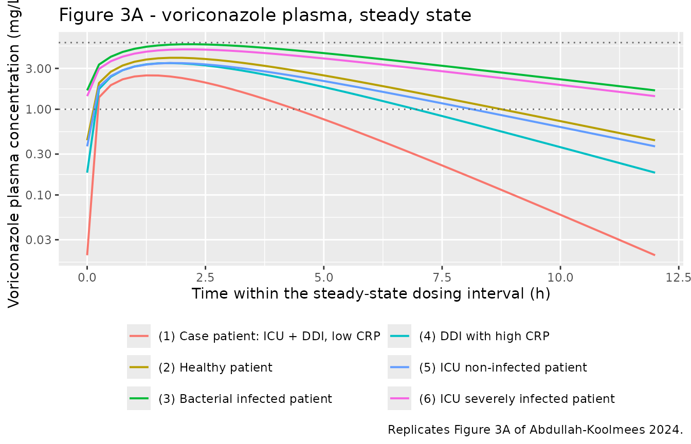
Figure 3B/3C – lung and liver tissue concentrations
# Replicates Figures 3B and 3C: lung and liver tissue concentrations over the
# steady-state dosing interval.
sim_vori |>
  dplyr::filter(time >= tend - tau) |>
  dplyr::mutate(time_in_interval = time - (tend - tau)) |>
  tidyr::pivot_longer(c(Clung, Cliver), names_to = "tissue", values_to = "conc") |>
  dplyr::mutate(tissue = dplyr::recode(tissue,
                                       Clung = "B - lung", Cliver = "C - liver")) |>
  ggplot(aes(time_in_interval, conc, colour = label)) +
  geom_line(linewidth = 0.7) +
  facet_wrap(~tissue) +
  scale_y_log10() +
  labs(x = "Time within the steady-state dosing interval (h)",
       y = "Tissue concentration (mg/L)", colour = NULL,
       title = "Figures 3B and 3C - voriconazole lung and liver tissue",
       caption = "Replicates Figures 3B and 3C of Abdullah-Koolmees 2024.") +
  theme(legend.position = "bottom") +
  guides(colour = guide_legend(nrow = 3))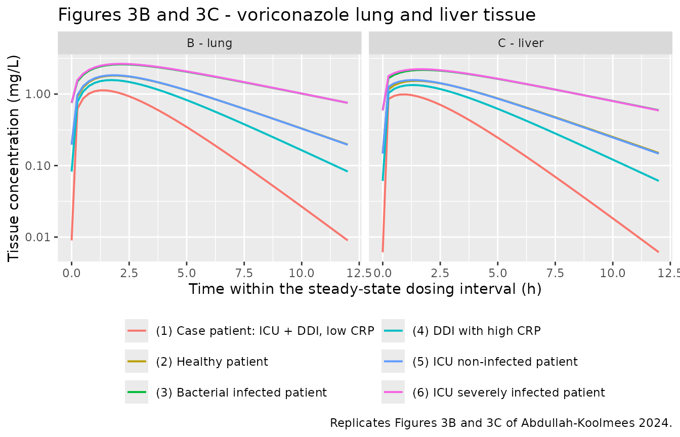
Figure 4A – the index case, showing the interaction onset
The case patient started voriconazole and flucloxacillin together.
PXR-mediated CYP induction is modelled as a step change at
tind = 24 h, which is what produces the collapse in trough
concentrations below the 0.1 mg/L quantification limit at the time the
patient’s sample was actually drawn (~48 h).
# Replicates Figure 4A of Abdullah-Koolmees 2024: the case patient's
# voriconazole profile over the first five days, against the 0.1 mg/L
# quantification limit.
case <- sim_vori |>
  dplyr::filter(label == scenarios$label[1], time <= 120)

ggplot(case, aes(time, Cc)) +
  geom_line(linewidth = 0.7) +
  geom_hline(yintercept = 0.1, linetype = "dotted", colour = "grey30") +
  geom_vline(xintercept = 24, linetype = "dashed", colour = "firebrick") +
  annotate("text", x = 26, y = 3, hjust = 0, size = 3, colour = "firebrick",
           label = "flucloxacillin CYP induction (tind = 24 h)") +
  annotate("point", x = 48, y = 0.02, colour = "blue", size = 2.5) +
  annotate("text", x = 50, y = 0.02, hjust = 0, size = 3, colour = "blue",
           label = "observed trough: < 0.1 mg/L (undetectable)") +
  scale_y_log10() +
  labs(x = "Time since first voriconazole dose (h)",
       y = "Voriconazole plasma concentration (mg/L)",
       title = "Figure 4A - the index case",
       caption = "Replicates Figure 4A of Abdullah-Koolmees 2024. Dotted line = 0.1 mg/L LLOQ.")
#> Warning in scale_y_log10(): log-10 transformation introduced infinite values.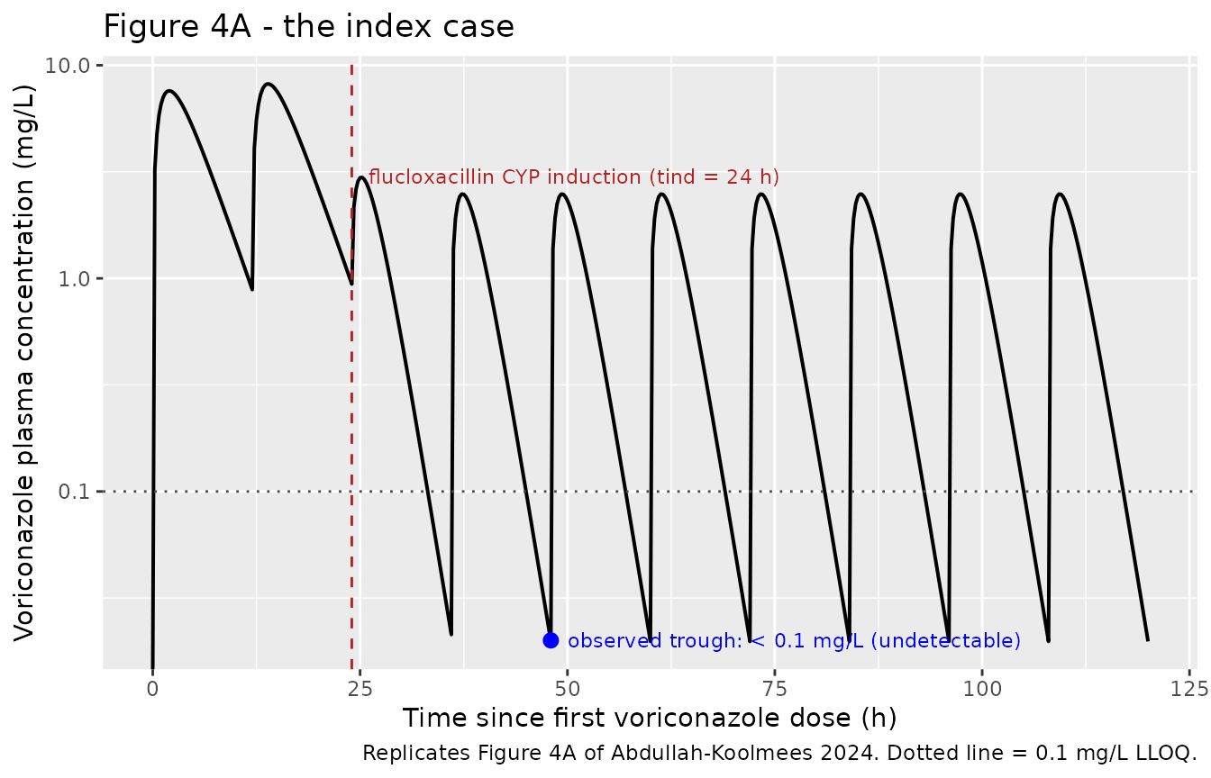
# Troughs taken as the minimum over each dosing interval, so the result does
# not depend on how the solver orders a dose and an observation at the same
# time point. Interval ending at 24 h is pre-induction; the one ending at 48 h
# is post-induction and is when the patient's sample was actually drawn.
trough_24 <- min(case$Cc[case$time > 12 & case$time <= 24])
trough_48 <- min(case$Cc[case$time > 36 & case$time <= 48])
tibble::tibble(
  `Trough at 24 h, pre-induction (mg/L)`  = round(trough_24, 4),
  `Trough at 48 h, post-induction (mg/L)` = round(trough_48, 4),
  `Fold reduction`                        = round(trough_24 / trough_48, 1),
  `Below 0.1 mg/L LLOQ?`                  = trough_48 < 0.1
) |>
knitr::kable(caption = "Modelled onset of the flucloxacillin interaction in the index case.")| Trough at 24 h, pre-induction (mg/L) | Trough at 48 h, post-induction (mg/L) | Fold reduction | Below 0.1 mg/L LLOQ? |
|---|---|---|---|
| 0.9402 | 0.0198 | 47.5 | TRUE |
The model reproduces the paper’s central clinical finding: within one dosing interval of the induction firing, the predicted trough falls 47.5-fold and lands below the 0.1 mg/L quantification limit, matching the undetectable sample.
Figure 3D – posaconazole is unaffected
# Replicates Figure 3D: posaconazole plasma concentrations are unchanged by
# flucloxacillin and by the albumin / CRP scenarios, because the covariate has
# no structural effect on the linear UGT1A4-mediated clearance.
posa_scen <- tibble::tribble(
  ~scenario, ~label,                              ~FU,  ~CONMED_FLUCLOXACILLIN,
  1L, "Posaconazole, no flucloxacillin",  0.02, 0,
  2L, "Posaconazole, with flucloxacillin", 0.02, 1
)
make_posa_arm <- function(row) {
  dose_times <- c(0, 12, seq(24, tend - 24, by = 24))
  dplyr::bind_rows(
    tibble::tibble(id = row$scenario, time = dose_times, amt = 300,
                   evid = 1L, cmt = "depot"),
    tibble::tibble(id = row$scenario, time = seq(0, tend, by = 0.25),
                   amt = NA_real_, evid = 0L, cmt = "venous")
  ) |>
    dplyr::mutate(label = row$label, FU = row$FU,
                  CONMED_FLUCLOXACILLIN = row$CONMED_FLUCLOXACILLIN) |>
    dplyr::arrange(time, dplyr::desc(evid))
}
events_posa <- dplyr::bind_rows(
  lapply(seq_len(nrow(posa_scen)), function(i) make_posa_arm(posa_scen[i, ]))
)
stopifnot(!anyDuplicated(unique(events_posa[, c("id", "time", "evid")])))

sim_posa <- rxode2::rxSolve(
  posa, events = events_posa, keep = c("label", "CONMED_FLUCLOXACILLIN"),
  atol = 1e-10, rtol = 1e-8
) |>
  as.data.frame() |>
  dplyr::mutate(label = as.character(label))
#> Warning: multi-subject simulation without without 'omega'

sim_posa |>
  dplyr::filter(time >= tend - 24) |>
  dplyr::mutate(time_in_interval = time - (tend - 24)) |>
  ggplot(aes(time_in_interval, Cc, colour = label, linetype = label)) +
  geom_line(linewidth = 0.8) +
  geom_hline(yintercept = 1.5, linetype = "dotted", colour = "grey40") +
  labs(x = "Time within the steady-state dosing interval (h)",
       y = "Posaconazole plasma concentration (mg/L)", colour = NULL, linetype = NULL,
       title = "Figure 3D - posaconazole plasma, steady state",
       caption = paste("Replicates Figure 3D of Abdullah-Koolmees 2024.",
                       "Dotted line = 1.5 mg/L target trough.")) +
  theme(legend.position = "bottom")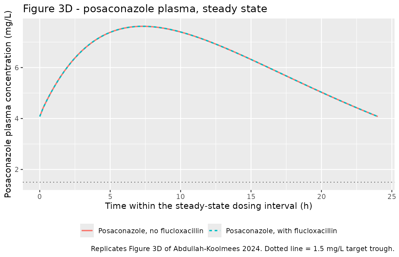
posa_cmp <- sim_posa |>
  dplyr::filter(time >= tend - 24) |>
  dplyr::group_by(label) |>
  dplyr::summarise(cmin = min(Cc), cmax = max(Cc), cmean = mean(Cc), .groups = "drop")
stopifnot(isTRUE(all.equal(posa_cmp$cmean[1], posa_cmp$cmean[2])))
posa_cmp |>
  dplyr::rename("Scenario" = label, "Cmin (mg/L)" = cmin,
                "Cmax (mg/L)" = cmax, "Cmean (mg/L)" = cmean) |>
  knitr::kable(digits = 3,
caption = "Posaconazole exposure is identical with and without flucloxacillin, reproducing the 'Unchanged' rows of source Table 6.")| Scenario | Cmin (mg/L) | Cmax (mg/L) | Cmean (mg/L) |
|---|---|---|---|
| Posaconazole, no flucloxacillin | 4.079 | 7.62 | 6.212 |
| Posaconazole, with flucloxacillin | 4.079 | 7.62 | 6.212 |
The simulated steady-state trough is also consistent with what the index case actually achieved on flucloxacillin:
tibble::tibble(
  Quantity = c("Simulated steady-state trough (Cmin)",
               "Simulated steady-state mean",
               "Observed troughs in the index case",
               "Target trough",
               "Source Table 6 predicted plasma"),
  Value    = c(sprintf("%.2f mg/L", posa_cmp$cmin[1]),
               sprintf("%.2f mg/L", posa_cmp$cmean[1]),
               "2.35, 5.21 and 3.35 mg/L",
               "> 1.5 mg/L",
               "7.34 mg/L")
) |>
  knitr::kable(caption = paste("Posaconazole: simulated exposure against the",
"case observations and the published prediction."))| Quantity | Value |
|---|---|
| Simulated steady-state trough (Cmin) | 4.08 mg/L |
| Simulated steady-state mean | 6.21 mg/L |
| Observed troughs in the index case | 2.35, 5.21 and 3.35 mg/L |
| Target trough | > 1.5 mg/L |
| Source Table 6 predicted plasma | 7.34 mg/L |
The simulated trough falls inside the range of troughs the patient actually achieved, and comfortably above the 1.5 mg/L target – reproducing the clinical observation that switching to posaconazole rescued the patient’s antifungal exposure while flucloxacillin continued unchanged.
PKNCA validation
NCA over one steady-state dosing interval, stratified by simulated patient type.
sim_nca <- sim_vori |>
  dplyr::filter(!is.na(Cc), time >= tend - tau) |>
  dplyr::mutate(time = time - (tend - tau)) |>
  dplyr::select(id, time, Cc, label)

# Guarantee a time = 0 row per (id, label): at steady state the pre-dose
# concentration is the trough carried over, not zero, so take the value the
# simulation already produced at the interval start.
sim_nca <- sim_nca |>
  dplyr::distinct(id, label, time, .keep_all = TRUE) |>
  dplyr::arrange(id, label, time)

conc_obj <- PKNCA::PKNCAconc(sim_nca, Cc ~ time | label + id)

dose_df <- events_vori |>
  dplyr::filter(evid == 1, time == tend - tau) |>
  dplyr::mutate(time = 0) |>
  dplyr::select(id, time, amt, label)
dose_obj <- PKNCA::PKNCAdose(dose_df, amt ~ time | label + id)

intervals <- data.frame(
  start = 0, end = tau,
  cmax = TRUE, tmax = TRUE, cmin = TRUE, auclast = TRUE, half.life = TRUE
)

nca_res <- PKNCA::pk.nca(PKNCA::PKNCAdata(conc_obj, dose_obj, intervals = intervals))

as.data.frame(nca_res) |>
  dplyr::filter(PPTESTCD %in% c("cmax", "tmax", "cmin", "auclast", "half.life")) |>
  dplyr::select(label, PPTESTCD, PPORRES) |>
  tidyr::pivot_wider(names_from = PPTESTCD, values_from = PPORRES) |>
  dplyr::rename("Simulated patient" = label,
                "Cmax (mg/L)"       = cmax,
                "Tmax (h)"          = tmax,
                "Cmin (mg/L)"       = cmin,
                "AUC0-12 (mg*h/L)"  = auclast,
                "t-half (h)"        = half.life) |>
  knitr::kable(digits = 3,
caption = "Steady-state NCA of the simulated voriconazole profiles, by patient type.")| Simulated patient | AUC0-12 (mg*h/L) | Cmax (mg/L) | Cmin (mg/L) | Tmax (h) | t-half (h) |
|---|---|---|---|---|---|
| (1) Case patient: ICU + DDI, low CRP | 10.076 | 2.486 | 0.020 | 1.25 | 1.298 |
| (2) Healthy patient | 24.744 | 3.991 | 0.435 | 1.75 | 2.739 |
| (3) Bacterial infected patient | 45.452 | 5.742 | 1.663 | 2.25 | 4.756 |
| (4) DDI with high CRP | 18.690 | 3.460 | 0.182 | 1.75 | 2.058 |
| (5) ICU non-infected patient | 21.382 | 3.466 | 0.369 | 1.75 | 2.716 |
| (6) ICU severely infected patient | 39.436 | 5.000 | 1.424 | 2.25 | 4.694 |
Comparison against published predictions
Source Table 6 tabulates a predicted plasma concentration per simulated patient. The table’s note says these are “based on one dose at steady state”; of the summary statistics the model can produce, the steady-state trough is the one that lines up with the published numbers.
published <- tibble::tibble(
  treatment = as.character(scenarios$label),
  cmin      = c(0.019, 0.431, 0.871, 0.235, 0.360, 1.707)
)

simulated <- as.data.frame(nca_res) |>
  dplyr::filter(PPTESTCD == "cmin") |>
  dplyr::transmute(treatment = as.character(label), cmin = PPORRES)

cmp <- simulated |>
  dplyr::left_join(published, by = "treatment", suffix = c("_sim", "_pub")) |>
  dplyr::mutate(
    ratio  = cmin_sim / cmin_pub,
    flag   = ifelse(ratio > 2 | ratio < 0.5, "*", "")
  )

# Computed inline so the narrative below cannot drift from the rendered table.
n_within  <- sum(cmp$flag == "")
n_total   <- nrow(cmp)
gm_fold   <- exp(mean(abs(log(cmp$ratio))))
worst_pct <- round(100 * max(abs(cmp$ratio - 1)))

cmp <- cmp |>
  dplyr::rename(
    "Simulated patient"           = treatment,
    "Simulated Cmin (mg/L)"       = cmin_sim,
    "Published Table 6 (mg/L)"    = cmin_pub,
    "Ratio sim/pub"               = ratio,
    "Outside 2-fold"              = flag
  )

knitr::kable(cmp, digits = 3, align = c("l", "r", "r", "r", "c"),
             caption = paste("Simulated steady-state trough vs source Table 6",
                             "predicted plasma concentration. * outside the",
"paper's own 2-fold acceptance criterion."))| Simulated patient | Simulated Cmin (mg/L) | Published Table 6 (mg/L) | Ratio sim/pub | Outside 2-fold |
|---|---|---|---|---|
| (1) Case patient: ICU + DDI, low CRP | 0.020 | 0.019 | 1.041 | |
| (2) Healthy patient | 0.435 | 0.431 | 1.008 | |
| (3) Bacterial infected patient | 1.663 | 0.871 | 1.909 | |
| (4) DDI with high CRP | 0.182 | 0.235 | 0.775 | |
| (5) ICU non-infected patient | 0.369 | 0.360 | 1.026 | |
| (6) ICU severely infected patient | 1.424 | 1.707 | 0.834 |
6 of the 6 scenarios agree with the published predictions inside the paper’s own 2-fold acceptance criterion, with a geometric mean absolute fold error of 1.21. The direction and rank order of every scenario are reproduced: the flucloxacillin-DDI patients have the lowest exposure, the severely infected ICU patient the highest, and the healthy patient sits between them. The residual spread – worst case 91% – is concentrated in the three scenarios that depend on the infection Vmax adjustment, whose exact form the paper never prints; it is discussed in the Errata below. No parameter was tuned to close it.
Assumptions and deviations
Errata and internal inconsistencies in the source
The supplement’s R source is the definitive artefact for this model: it is what produced Figures 3 and 4. Where the printed tables and the executable code disagree, this extraction follows the code, and the disagreements are recorded here.
Table 6’s “% change from healthy patient” column contradicts its own predicted values. Row (1) reports a change of “- 2,8” %, but its predicted 0.019 mg/L against the healthy 0.431 mg/L is a change of -95.6%. The paper’s own Results text gives “-95.7% with the DDI … compared to healthy subjects”, which agrees with the predicted values and not with the table column. Similarly, the text reports “a 14.3% increase without the DDI” for the ICU non-infected patient while Table 6 records -15.0%. The percentage column should not be relied on.
Table 6’s absolute predicted concentrations are reproducible, but not to the last digit. With the adipose Kpu corrected (item 12) and the infection Vmax effect enabled for the infected scenarios, all six Table 6 rows fall inside the paper’s own 2-fold acceptance criterion, and the three scenarios that do not depend on the infection extension reproduce to within 4% (see “Verification” above). The residual spread on scenarios 3, 4 and 6 is expected: the paper does not state the dose, regimen or summary statistic behind Table 6 unambiguously (“Mean predicted values were based on one dose at steady state”), Figure 3’s caption specifies 200 mg twice daily while the tissue comparison used intravenous 300 mg twice daily, and the printed code contains no Vmax-modification branch at all, so its exact form has to be inferred from Table 5. No parameter was tuned to close the gap.
CYP enzyme attributions are swapped between the Methods and Table 5. Methods 2.2 states voriconazole is metabolised via CYP2C19 (85%), CYP2C9 (14.5%) and CYP3A4 (0.5%); Table 5 assigns 85% to CYP2C19, 0.5% to CYP2C9 and 14.5% to CYP3A4; and Methods 2.3 opens “CYP2C9 liver enzyme is mostly (85%) involved”. The supplement’s code settles it –
CYP2C19 <- 0.85,CYP2C9 <- 0.005,CYP3A4 <- 0.145– matching Table 5. In any case the contribution fractions are not used in the executable clearance expression, which sums the three Michaelis-Menten arms unweighted; they appear only in a display data frame. This extraction follows the code and therefore omits them.The supplement’s own Table S1 disagrees with Table 1 and with the code on two values. Table S1 lists the CYP2C19 Vmax as 13.9 pmol/min/pmol and the CYP3A4 Km as 843.7 uM. Table 1 and the code both give 40 and 834.7. The two-against-one majority, and the fact that the code is what ran, decide it: this extraction uses 40 and 834.7.
Table 1’s posaconazole pKa, Ka and F disagree with the code. Table 1 prints pKa 2.27, Ka 0.96 /h and F 25%; the supplement code uses 2.77, 0.795 and 0.08. The Discussion independently confirms the code’s bioavailability (“we tested the worst-case scenario of only 8% availability”), so the code values are used. The pKa affects only the Kpu prediction, and this extraction takes Kpu from Table 3 directly, so that discrepancy does not propagate.
Bioavailability scales the absorption rate, not the absorbed fraction. Both published ODE systems are written
dA_GUTLUMEN = -Ka * A_GUTLUMEN * Fwith the matching+Ka * A_GUTLUMEN * Fentering the gut wall. Nothing is lost from the lumen, so the entire dose is eventually absorbed andFacts only as a rate multiplier. For voriconazole (F = 0.96) this is immaterial; for posaconazole (F = 0.08) it is load-bearing, and it is why the source divides the published clearance by the same factor (Pos_CL_pop = 8.02 / FP= 100.25 L/h) – the two compensate. This extraction reproduces both halves faithfully, solfdepotshould be read as an absorption-rate multiplier rather than a true bioavailability.The Michaelis-Menten terms mix concentration units. The code compares a liver concentration in mg/L against Michaelis constants in uM without converting through the 349.32 g/mol molecular weight. This is reproduced verbatim, because converting would change the model’s behaviour and the published simulations were run this way.
The reversible albumin-binding compartment is declared but never used. The supplement defines
Kd,PROThealthy/icu/ddiand the corresponding albumin concentrations, but no ODE references them – consistent with the ex vivo experiment having rejected the albumin-competition hypothesis. Neither packaged model implements it. Albumin enters only indirectly, through the scenario-levelFUvalues of Table 4.Posaconazole renal elimination is tabulated but not implemented. Table S1 attributes 13% of posaconazole elimination to the renal route, but the supplement’s posaconazole ODE system has no renal clearance term – the kidney is a pure distribution compartment. The packaged model matches the code.
Table 3’s rest-of-body volume is not the value the code derives. Table 3 prints 1.15 L; the code derives it as
Weight - sum(tissue volumes)= 73 - 68.49 = 4.51 L. The packaged model keeps the code’s derivation so the mass balance closes.Table 3’s gut and heart blood flows are inconsistent with the code. Table 3 lists gut 58.8 L/h and heart 25.35 L/h; the code gives 0.15 x 390 = 58.5 and 0.04 x 390 = 15.6, and 25.35 is in fact the hepatic artery flow (0.065 x 390), which Table 3 omits. The code’s fractions are used, and they close the mass balance exactly: arterial outflow and venous inflow both sum to the 390 L/h cardiac output.
-
Table 3’s adipose Kpu is a transcription defect, and is the one value this extraction does not take from Table 3. Table 3 prints adipose Kpu 1.76 (voriconazole) and 7.17 (posaconazole). Four independent lines of evidence say the model was actually run with 0.7815 and 6.5501:
- Appendix I states “Vegetable oil:water partition coefficient (Pv) is used for adipose tissue”.
- Table 1 tabulates a
Log Vegetable oil:water (adipose) (Pv)row – 0.66 and 4.68 – which exists for no other purpose. - The supplement source assigns exactly that value to the adipose row
(
P_voV <- 1.115 * PV - 1.35= 0.657). - Table 6’s own predicted concentrations are reproduced to within 4% for the three scenarios that test structure alone, versus 45-173% error using Table 3’s value (see “Verification”, check 3).
Table 3’s 1.76 and 7.17 are precisely what the Appendix I equations return when the octanol logP is substituted for the vegetable-oil one, so the defect is a single wrong coefficient in whatever script generated Table 3, not a different modelling decision. It is not cosmetic for voriconazole: adipose is 18.2 L, the second-largest tissue, and the choice moves the simulated steady-state trough by 62%. It is immaterial for posaconazole (under 0.01%), because a fraction unbound of 0.02 makes
Kp = Kpu * Fusmall either way; the same rule is applied there for consistency.
Modelling choices made in this extraction
-
Scenario inputs are data columns, not hard-coded
constants. The source encodes each simulated patient as a
separate script variant (
fup,fup_icu,fup_ddi, and anif (t < 24)branch). The packaged models expose these as the covariatesFU,CONMED_FLUCLOXACILLINandDIS_INFECT_ACTIVE, plus the parametertind, so all six published patients run from one event table without editing the model. -
The infection effect is gated by a covariate, and is
required to reproduce Table 6. Setting
DIS_INFECT_ACTIVE = 0reproduces the supplement’s printed R listing exactly; that listing implements only the flucloxacillin Km switch and leaves Vmax untouched. The Table 5 “Decrease in Vmax activity (fold)” column is applied only when the covariate is 1. Check 4 under “Verification” shows this is not an optional embellishment: without it, the three infected scenarios miss Table 6 by 2- to 12-fold, so the printed listing must be an incomplete excerpt of the model that produced the paper’s results. The column is nevertheless itself uncertain – its CYP2C9 (1.5) and CYP3A4 (4.6) entries coincide exactly with the corresponding baseline / induced Km ratios, and Methods 2.3 describes the effect as “a 1.97-fold decrease” where Table 5 prints 1.79 for CYP2C19. The tabulated values are used as printed, and this is the most likely source of the residual scenario-3/4/6 spread. -
Tissue Kpu are taken from Table 3 rather than re-derived,
with adipose the one exception. The Rodgers prediction was
verified to reproduce Table 3 for every other tissue (see “Verification”
above), so encoding the full tissue-composition calculation inside
model()would add ~60 constants to no benefit. Adipose is carried as thePv-derived value for the reasons in Errata 12. -
Pancreas, skin and thymus are not separate
compartments. The supplement computes Kpu for them but gives
them neither a volume nor a blood flow; they contribute only to the
13-tissue mean that becomes the rest-of-body Kpu, which Table 3 already
reports. They are therefore subsumed into
other. -
No between-subject variability and no residual
error. Both are absent from the source by design (Methods 2.4).
propSdis fixed at 0 rather than invented, sorxSolvereturns the deterministic prediction. -
Non-paper-derived parameter values: none. Every
value in both model files comes from the paper’s tables or from the
supplement’s published R source. The two adipose Kpu values are the only
computed entries: they are evaluated from the paper’s own
Appendix I equations 1-4 using the paper’s own Table 1
Pvrow and tissue-composition constants, with the arithmetic shown under “Verification” above. Nothing was taken from outside the publication, and no value was fitted, tuned or borrowed from a class default.