Darunavir (Tsirizani 2024)
Source:vignettes/articles/Tsirizani_2024_darunavir.Rmd
Tsirizani_2024_darunavir.RmdModel and source
- Citation: Tsirizani L, Mohsenian Naghani S, Waalewijn H, Szubert A, Mulenga V, Chabala C, Bwakura-Dangarembizi M, Chitsamatanga M, Rutebarika DA, Musiime V, Kasozi M, Lugemwa A, Monkiewicz LN, McIlleron HM, Burger DM, Gibb DM, Denti P, Wasmann RE, Colbers A; the CHAPAS-4 trial team. Pharmacokinetics of once-daily darunavir/ritonavir in second-line treatment in African children with HIV. J Antimicrob Chemother. 2024;79(11):2990-2998. doi:10.1093/jac/dkae319. Parameter values from Table 3 and its footnote c (the clearance-AAG equation).
- Description (final model): Two-compartment population PK model for oral darunavir boosted with ritonavir (600/100 or 800/100 mg once daily) in African children with HIV on second-line ART (CHAPAS-4 trial PK sub-study; 59 children aged 3.8-14.7 years and 14.5-47.0 kg from Zambia, Uganda and Zimbabwe). Absorption is a Savic transit-compartment chain (mean transit time MTT, non-integer number of transit compartments NN) feeding an absorption compartment drained first-order at ka. Clearance and both volumes are allometrically scaled to total body weight with exponents fixed at 0.75 and 1, referenced to 26 kg. Plasma alpha-1-acid glycoprotein (AAG) lowers apparent clearance exponentially (slope -0.582 per g/L around 0.66 g/L). Between-subject variability on clearance only; between-occasion variability on bioavailability, MTT and ka. No effect of the NRTI backbone (tenofovir alafenamide/emtricitabine, abacavir/lamivudine or zidovudine/lamivudine), age or ritonavir exposure was retained. All clearances and volumes are apparent (/F).
- Description (supplementary AAG-binding model): Semi-mechanistic two-compartment population PK model for oral darunavir boosted with ritonavir in African children with HIV on second-line ART (CHAPAS-4 PK sub-study; 59 children, 14.5-47.0 kg), with saturable instantaneous binding of darunavir to alpha-1-acid glycoprotein (AAG) in the central compartment. Bound darunavir follows Cbound = Bmax * Cfree / (Kd + Cfree), and the AAG binding capacity Bmax rises with plasma AAG through a power relationship (exponent 0.405, reference 0.7 g/L). Only free darunavir is cleared (intrinsic clearance CLint) and distributes to the peripheral compartment; the observation is total plasma darunavir. Absorption is a Savic transit chain feeding an absorption compartment drained at ka; clearances and volumes scale allometrically with weight (exponents fixed 0.75 and 1, reference 26 kg). This is the alternative model reported in the supplement; the authors adopted the simpler direct AAG-on-clearance model (Tsirizani_2024_darunavir) for parsimony and usability.
- Article: https://doi.org/10.1093/jac/dkae319 (open access, PMC11531812)
Tsirizani 2024 reports two fits to the same CHAPAS-4 darunavir data.
The final model (Table 3), packaged as
Tsirizani_2024_darunavir, lets plasma alpha-1-acid
glycoprotein (AAG) lower apparent clearance directly. A semi-mechanistic
alternative (Supplementary Table 1 and Supplementary Figure 2), packaged
as Tsirizani_2024_darunavir_aagbinding, instead binds
darunavir saturably to AAG and clears only the free drug; it fitted
better (dOFV = 11) but the authors kept the simpler model for parsimony
and usability. Both are shipped so that the binding description can be
used where unbound exposure matters.
The companion ritonavir model from the same trial is
Tsirizani_2025_ritonavir.
Population
Fifty-nine children aged 3.8-14.7 years (median 10.9) weighing 14.5-47.0 kg (median 26.0), 55.9% female, from Zambia, Uganda and Zimbabwe, were randomised to the darunavir/ritonavir arm of CHAPAS-4 after failing first-line abacavir- or zidovudine-based ART (Table 1). Darunavir/ritonavir was given once daily by weight band: 600/100 mg at 14-24.9 kg and 800/100 mg at 25 kg or more (17.0-41.4 mg/kg darunavir). The NRTI backbone was tenofovir alafenamide/emtricitabine (N = 34), abacavir/lamivudine (N = 12) or zidovudine/lamivudine (N = 13). Median AAG was 0.7 g/L (0.3-1.9). Intensive steady-state sampling at week 6 followed a witnessed dose taken with breakfast, at pre-dose and 1, 2, 4, 6, 8, 12 and 24 h (plus 0.5 h in the TAF arm); 491 darunavir concentrations were analysed in NONMEM 7.5.1 with FOCE-I.
The same information is available programmatically via
readModelDb("Tsirizani_2024_darunavir")()$population.
Source trace
Every ini() value carries an in-file comment naming its
source row. The table collects them.
Final model (Tsirizani_2024_darunavir)
| Equation / parameter | Value | Source location |
|---|---|---|
lcl (CL/F at 26 kg, AAG 0.66 g/L) |
log(8.05) L/h | Table 3 |
lvc (Vc/F at 26 kg) |
log(46.3) L | Table 3 |
lq (Q/F at 26 kg) |
log(7.79) L/h | Table 3 |
lvp (Vp/F at 26 kg) |
log(82.6) L | Table 3 |
lfdepot |
fixed(log(1)) | Table 3 (‘1 FIXED’) |
lmtt |
log(0.763) h | Table 3 |
lnn |
log(11.6) | Table 3 |
lka |
log(0.551) 1/h | Table 3 |
e_wt_cl_q, e_wt_vc_vp
|
fixed 0.75, 1 | Methods, ‘Population pharmacokinetic analysis’; Table 3 footnote b (26 kg reference) |
e_aag_cl |
-0.582 per g/L | Table 3; footnote c
CL = 8.05 (WT/26)^0.75 exp(-0.582 (AAG - 0.66))
|
etalcl |
0.324^2 | Table 3, BSV clearance 32.4% |
etaiov_fdepot_*, etaiov_mtt_*,
etaiov_ka_*
|
0.444^2, 0.608^2, 0.434^2 | Table 3, BOV 44.4%, 60.8%, 43.4% |
propSd, addSd
|
0.125, 0.291 mg/L | Table 3 residual error |
| Two-compartment disposition | n/a | Results, ‘Population pharmacokinetic analysis’ (dOFV 40.3 vs one compartment) |
Transit absorption, ktr = (NN + 1) / MTT
|
n/a | Results (transit compartments, dOFV 269.8); Methods reference 22 (Savic 2007) |
Supplementary binding model
(Tsirizani_2024_darunavir_aagbinding)
| Equation / parameter | Value | Source location |
|---|---|---|
lclint (CLint/F at 26 kg) |
log(97.7) L/h | Supplementary Table 1 |
lvc |
log(40.6) L | Supplementary Table 1 |
lq |
log(62.7) L/h | Supplementary Table 1 |
lvp |
log(822) L | Supplementary Table 1 |
lfdepot |
fixed(log(1)) | Supplementary Table 1 |
lmtt, lnn, lka
|
log(0.849) h, log(5.31), log(0.519) 1/h | Supplementary Table 1 |
lkd |
log(1.31) mg/L | Supplementary Table 1 |
lbmax |
log(20.7) mg/L | Supplementary Table 1 |
e_aag_bmax |
0.405 | Supplementary Table 1 and footnote #
Bmax = 20.7 (AAG/0.7)^0.405
|
etalclint |
0.351^2 | Supplementary Table 1, BSV 35.1% |
etaiov_fdepot_*, etaiov_mtt_*,
etaiov_ka_*
|
0.470^2, 0.624^2, 0.387^2 | Supplementary Table 1, BOV 47.0%, 62.4%, 38.7% |
propSd, addSd
|
0.127, 0.337 mg/L | Supplementary Table 1 |
Cbound = Bmax Cfree / (Kd + Cfree); free drug
eliminated and distributed |
n/a | Supplementary Figure 2 and its caption |
Typical-value checks
Two deterministic identities pin the encoding before any cohort is
drawn. Because the transit chain delivers the dose through a closed-form
input (podo() / tad()), the first check
confirms the whole bioavailable dose reaches the system: for the final
model, a single dose must give AUC(0-inf) = Dose / CL. For the binding
model, only free drug is cleared, so at steady state the free AUC over
one interval must equal Dose / CLint.
mod_final <- readModelDb("Tsirizani_2024_darunavir")
mod_bind <- readModelDb("Tsirizani_2024_darunavir_aagbinding")

grid_sd <- seq(0, 480, by = 0.1)
ev_sd <- dplyr::bind_rows(
  data.frame(id = 1L, time = 0, evid = 1L, amt = 800, cmt = "depot"),
  data.frame(id = 1L, time = grid_sd, evid = 0L, amt = 0, cmt = "central")
) |>
  dplyr::mutate(WT = 26, AAG = 0.66, OCC = 2L)

trap <- function(t, y) sum(diff(t) * (head(y, -1) + tail(y, -1)) / 2)

sd_final <- rxode2::rxSolve(rxode2::zeroRe(mod_final), ev_sd,
                            rtol = 1e-10, atol = 1e-12) |>
  as.data.frame()
#> ℹ parameter labels from comments will be replaced by 'label()'
#> Warning: some etas defaulted to non-mu referenced, possible parsing error: etaiov_fdepot_1, etaiov_fdepot_2, etaiov_mtt_1, etaiov_mtt_2, etaiov_ka_1, etaiov_ka_2
#> as a work-around try putting the mu-referenced expression on a simple line
#> Warning: some etas defaulted to non-mu referenced, possible parsing error: etaiov_fdepot_1, etaiov_fdepot_2, etaiov_mtt_1, etaiov_mtt_2, etaiov_ka_1, etaiov_ka_2
#> as a work-around try putting the mu-referenced expression on a simple line
#> ℹ omega/sigma items treated as zero: 'etalcl', 'etaiov_fdepot_1', 'etaiov_fdepot_2', 'etaiov_mtt_1', 'etaiov_mtt_2', 'etaiov_ka_1', 'etaiov_ka_2'
auc_sd <- trap(sd_final$time, sd_final$Cc)
cl_typ <- 8.05
c(AUC_sim = auc_sd, Dose_over_CL = 800 / cl_typ)
#>      AUC_sim Dose_over_CL
#>     99.37888     99.37888
stopifnot(max(sd_final$Cc) > 1, abs(auc_sd / (800 / cl_typ) - 1) < 0.005)

# Steady state (7 daily doses), binding model: free AUC over the last
# interval x CLint = Dose.
ev_ss <- dplyr::bind_rows(
  data.frame(id = 1L, time = seq(0, 144, by = 24), evid = 1L, amt = 800,
             cmt = "depot"),
  data.frame(id = 1L, time = seq(144, 168, by = 0.05), evid = 0L, amt = 0,
             cmt = "central")
) |>
  dplyr::mutate(WT = 26, AAG = 0.7, OCC = 2L) |>
  dplyr::arrange(time, dplyr::desc(evid))

ss_bind <- rxode2::rxSolve(rxode2::zeroRe(mod_bind), ev_ss,
                           rtol = 1e-10, atol = 1e-12) |>
  as.data.frame()
#> ℹ parameter labels from comments will be replaced by 'label()'
#> Warning: some etas defaulted to non-mu referenced, possible parsing error: etaiov_fdepot_1, etaiov_fdepot_2, etaiov_mtt_1, etaiov_mtt_2, etaiov_ka_1, etaiov_ka_2
#> as a work-around try putting the mu-referenced expression on a simple line
#> Warning: some etas defaulted to non-mu referenced, possible parsing error: etaiov_fdepot_1, etaiov_fdepot_2, etaiov_mtt_1, etaiov_mtt_2, etaiov_ka_1, etaiov_ka_2
#> as a work-around try putting the mu-referenced expression on a simple line
#> ℹ omega/sigma items treated as zero: 'etalclint', 'etaiov_fdepot_1', 'etaiov_fdepot_2', 'etaiov_mtt_1', 'etaiov_mtt_2', 'etaiov_ka_1', 'etaiov_ka_2'
# Seven daily doses leave the slow free-drug peripheral pool short of full
# accumulation, so solve a long run-in instead for the free-drug balance.
ev_ss_long <- dplyr::bind_rows(
  data.frame(id = 1L, time = seq(0, 24 * 59, by = 24), evid = 1L, amt = 800,
             cmt = "depot"),
  data.frame(id = 1L, time = seq(24 * 59, 24 * 60, by = 0.05), evid = 0L,
             amt = 0, cmt = "central")
) |>
  dplyr::mutate(WT = 26, AAG = 0.7, OCC = 2L) |>
  dplyr::arrange(time, dplyr::desc(evid))
ss_bind_long <- rxode2::rxSolve(rxode2::zeroRe(mod_bind), ev_ss_long,
                                rtol = 1e-10, atol = 1e-12) |>
  as.data.frame()
#> ℹ parameter labels from comments will be replaced by 'label()'
#> Warning: some etas defaulted to non-mu referenced, possible parsing error: etaiov_fdepot_1, etaiov_fdepot_2, etaiov_mtt_1, etaiov_mtt_2, etaiov_ka_1, etaiov_ka_2
#> as a work-around try putting the mu-referenced expression on a simple line
#> Warning: some etas defaulted to non-mu referenced, possible parsing error: etaiov_fdepot_1, etaiov_fdepot_2, etaiov_mtt_1, etaiov_mtt_2, etaiov_ka_1, etaiov_ka_2
#> as a work-around try putting the mu-referenced expression on a simple line
#> ℹ omega/sigma items treated as zero: 'etalclint', 'etaiov_fdepot_1', 'etaiov_fdepot_2', 'etaiov_mtt_1', 'etaiov_mtt_2', 'etaiov_ka_1', 'etaiov_ka_2'
auc_free <- trap(ss_bind_long$time, ss_bind_long$Cu)
c(CLint_x_AUCfree = 97.7 * auc_free, Dose = 800)
#> CLint_x_AUCfree            Dose
#>             800             800
stopifnot(abs(97.7 * auc_free / 800 - 1) < 0.01)
Both identities hold. The binding model predicts an unbound fraction of 6.4-10.0% over a steady-state interval at the median AAG, falling as total concentration falls because binding is saturable.
ev_ss_typ <- ev_ss |>
  dplyr::mutate(AAG = 0.66)
ss_final <- rxode2::rxSolve(rxode2::zeroRe(mod_final), ev_ss_typ) |>
  as.data.frame()
#> ℹ parameter labels from comments will be replaced by 'label()'
#> Warning: some etas defaulted to non-mu referenced, possible parsing error: etaiov_fdepot_1, etaiov_fdepot_2, etaiov_mtt_1, etaiov_mtt_2, etaiov_ka_1, etaiov_ka_2
#> as a work-around try putting the mu-referenced expression on a simple line
#> Warning: some etas defaulted to non-mu referenced, possible parsing error: etaiov_fdepot_1, etaiov_fdepot_2, etaiov_mtt_1, etaiov_mtt_2, etaiov_ka_1, etaiov_ka_2
#> as a work-around try putting the mu-referenced expression on a simple line
#> ℹ omega/sigma items treated as zero: 'etalcl', 'etaiov_fdepot_1', 'etaiov_fdepot_2', 'etaiov_mtt_1', 'etaiov_mtt_2', 'etaiov_ka_1', 'etaiov_ka_2'
dplyr::bind_rows(
  dplyr::transmute(ss_final, model = "Final (Table 3)", tad = time - 144, Cc),
  dplyr::transmute(ss_bind, model = "AAG binding (Supplementary Table 1)",
                   tad = time - 144, Cc)
) |>
  ggplot(aes(tad, Cc, colour = model)) +
  geom_line(linewidth = 0.8) +
  labs(x = "Time after dose (h)", y = "Total darunavir (mg/L)", colour = NULL,
       title = "Typical 26 kg child, 800/100 mg once daily, steady state") +
  theme_bw() +
  theme(legend.position = "bottom")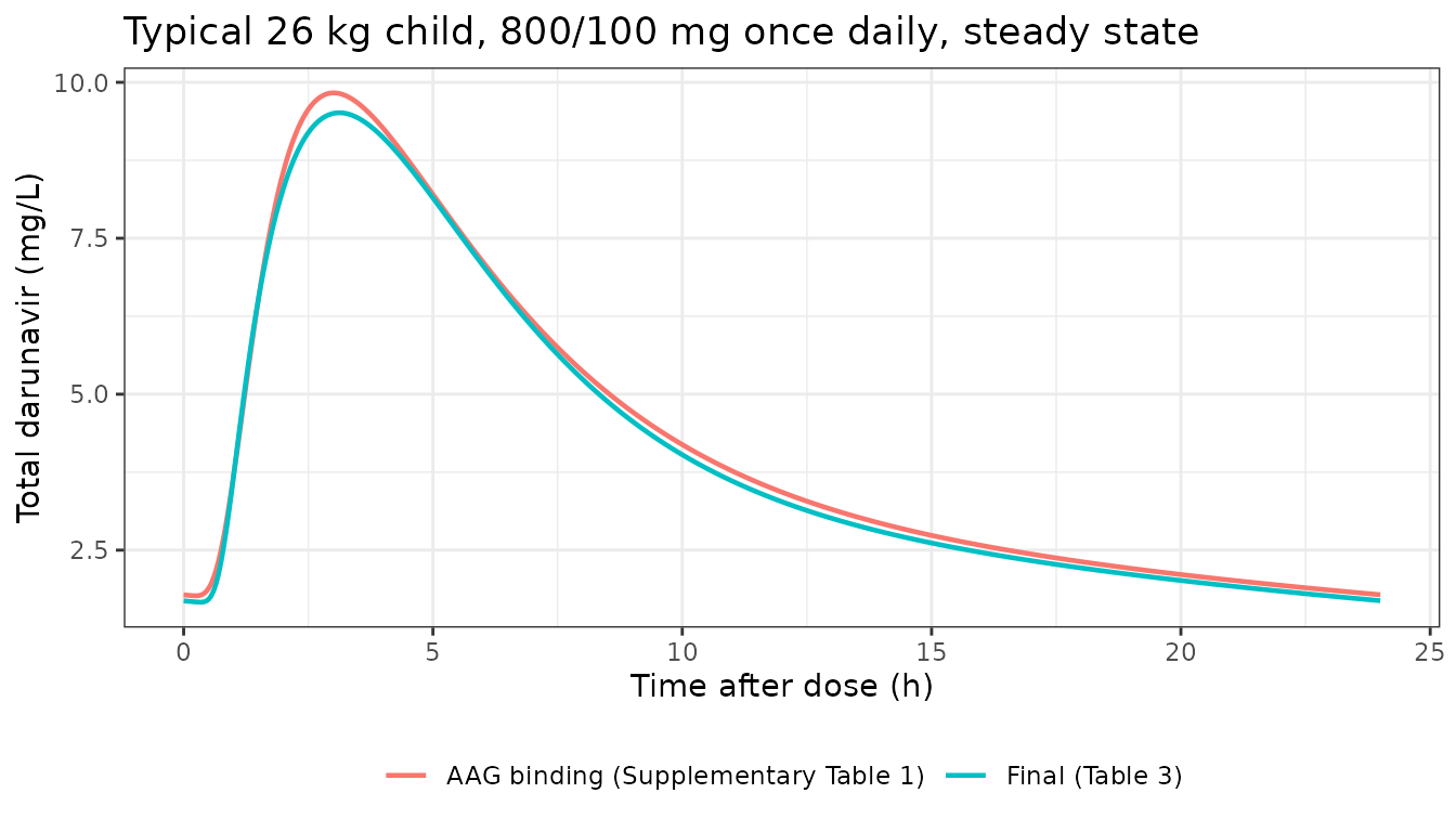
The two fits describe nearly the same total-concentration profile for a typical child, as expected for two models fitted to the same data.
Virtual cohort
The paper’s simulations (Figure 4) used a representative virtual population of 100,000 children dosed by weight band. Here each of the five Figure 4 arms gets 100 children. Weight is drawn uniformly within the band (the upper band capped at the observed maximum of 47 kg); AAG is drawn log-normally around the 0.7 g/L median with a log-scale SD of 0.35, clamped to the observed 0.3-1.9 g/L. Each child takes seven daily doses; the first six are occasion 1 and the seventh, witnessed dose and its 24 h profile are occasion 2.
set.seed(20241101)
rxode2::rxSetSeed(20241101)

arms <- tibble::tribble(
  ~arm,                       ~band,       ~wt_lo, ~wt_hi, ~dose,
  "14-19.9 kg, 600 mg",       "14-19.9",   14.5,   19.9,   600,
  "20-24.9 kg, 600 mg",       "20-24.9",   20,     24.9,   600,
  "25-34.9 kg, 600 mg (WHO)", "25-34.9",   25,     34.9,   600,
  "25-34.9 kg, 800 mg",       "25-34.9",   25,     34.9,   800,
  ">=35 kg, 800 mg",          ">=35",      35,     47,     800
)
n_per_arm <- 100L

cohort <- arms |>
  dplyr::mutate(arm_i = dplyr::row_number()) |>
  tidyr::uncount(n_per_arm) |>
  dplyr::mutate(
    id = dplyr::row_number(),
    WT = stats::runif(dplyr::n(), wt_lo, wt_hi),
    AAG = pmin(pmax(stats::rlnorm(dplyr::n(), log(0.7), 0.35), 0.3), 1.9)
  )

dose_times <- seq(0, 144, by = 24)
obs_tad <- seq(0, 24, by = 0.5)

events <- dplyr::bind_rows(
  tidyr::expand_grid(cohort, time = dose_times) |>
    dplyr::mutate(evid = 1L, amt = dose, cmt = "depot",
                  OCC = ifelse(time < 144, 1L, 2L)),
  tidyr::expand_grid(cohort, time = 144 + obs_tad) |>
    dplyr::mutate(evid = 0L, amt = 0, cmt = "central", OCC = 2L)
) |>
  dplyr::select(id, time, evid, amt, cmt, WT, AAG, OCC, arm, band) |>
  dplyr::arrange(id, time, dplyr::desc(evid))

stopifnot(
  !anyDuplicated(unique(events[, c("id", "time", "evid")])),
  max(table(cohort$arm)) <= 200
)
Simulation
sim <- rxode2::rxSolve(mod_final, events = events,
                       keep = c("arm", "band", "WT", "AAG")) |>
  as.data.frame() |>
  dplyr::mutate(tad = time - 144)
#> ℹ parameter labels from comments will be replaced by 'label()'
#> Warning: some etas defaulted to non-mu referenced, possible parsing error: etaiov_fdepot_1, etaiov_fdepot_2, etaiov_mtt_1, etaiov_mtt_2, etaiov_ka_1, etaiov_ka_2
#> as a work-around try putting the mu-referenced expression on a simple line
sim_bind <- rxode2::rxSolve(mod_bind, events = events,
                            keep = c("arm", "band", "WT", "AAG")) |>
  as.data.frame() |>
  dplyr::mutate(tad = time - 144)
#> ℹ parameter labels from comments will be replaced by 'label()'
#> Warning: some etas defaulted to non-mu referenced, possible parsing error: etaiov_fdepot_1, etaiov_fdepot_2, etaiov_mtt_1, etaiov_mtt_2, etaiov_ka_1, etaiov_ka_2
#> as a work-around try putting the mu-referenced expression on a simple line

stopifnot(
  all(is.finite(sim$Cc)), all(is.finite(sim_bind$Cc)),
  max(sim$Cc) > 1, max(sim_bind$Cc) > 1
)
Replicate published figures
Figure 1: median steady-state profiles by weight band
# Approximate medians of the 'Total' curve, read by the maintainers from
# Figure 1 of Tsirizani 2024 (observed data, all children).
fig1_total <- tibble::tibble(
  tad = c(0, 1, 2, 4, 6, 8, 12, 24),
  Cc = c(1.4, 4.2, 6.2, 8.5, 7.0, 5.0, 3.1, 2.0)
)

sim |>
  dplyr::filter(arm != "25-34.9 kg, 600 mg (WHO)") |>
  dplyr::group_by(band, tad) |>
  dplyr::summarise(Cc = stats::median(Cc), .groups = "drop") |>
  ggplot(aes(tad, Cc, colour = band)) +
  geom_line(linewidth = 0.8) +
  geom_point(data = fig1_total, aes(tad, Cc), inherit.aes = FALSE,
             shape = 16, size = 2.5) +
  labs(x = "Time after dose (h)", y = "Median darunavir (mg/L)",
       colour = "Weight band (kg)",
       caption = paste("Lines: simulated medians, CHAPAS-4 dosing.",
                       "Points: observed total medians read from Figure 1.")) +
  theme_bw()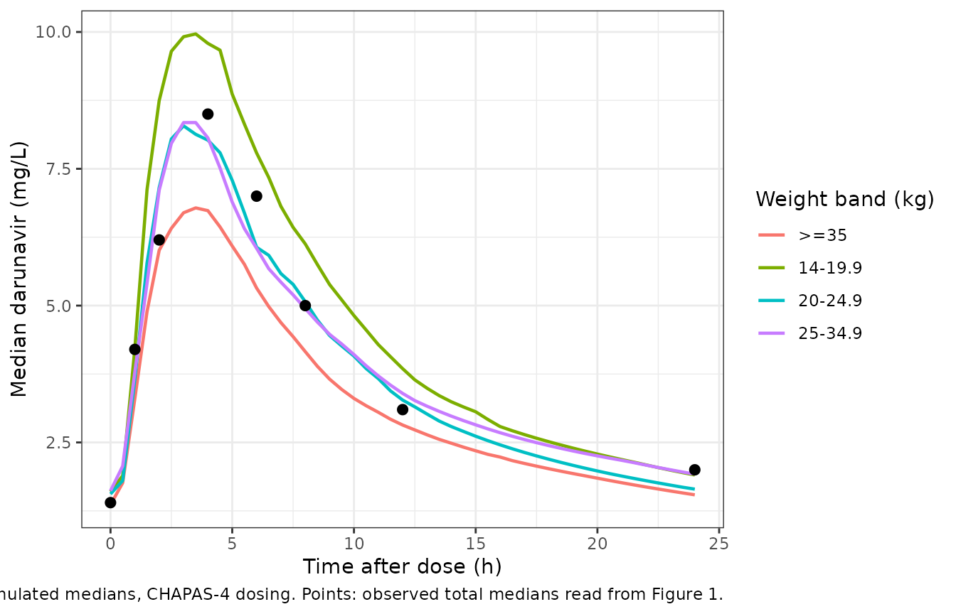
Replicates Figure 1 of Tsirizani 2024. The simulated medians peak at about 7-11 mg/L at 3-4 h, highest in the lightest band, and decline to 1.5-2 mg/L at 24 h, as observed.
Figure 4: simulated exposure by weight band
exposure <- function(s, model) {
  s |>
    dplyr::group_by(id, arm, band) |>
    dplyr::summarise(
      AUC = trap(tad, Cc),
      Cmax = max(Cc),
      Ctrough = Cc[tad == 24],
      .groups = "drop"
    ) |>
    dplyr::mutate(model = model)
}
expo <- dplyr::bind_rows(
  exposure(sim, "Final (Table 3)"),
  exposure(sim_bind, "AAG binding (Supplementary Table 1)")
)

# Medians read by the maintainers from the box plots of Figure 4.
fig4 <- tibble::tribble(
  ~arm,                       ~AUC, ~Cmax, ~Ctrough,
  "14-19.9 kg, 600 mg",       110,  10.5,  1.85,
  "20-24.9 kg, 600 mg",        88,   8.3,  1.55,
  "25-34.9 kg, 600 mg (WHO)",  71,   6.6,  1.35,
  "25-34.9 kg, 800 mg",        97,   8.8,  1.75,
  ">=35 kg, 800 mg",           77,   6.8,  1.45
)
expo_long <- expo |>
  dplyr::filter(model == "Final (Table 3)") |>
  tidyr::pivot_longer(c(AUC, Cmax, Ctrough), names_to = "metric")
fig4_long <- fig4 |>
  tidyr::pivot_longer(c(AUC, Cmax, Ctrough), names_to = "metric")
box_stats <- expo_long |>
  dplyr::group_by(arm, metric) |>
  dplyr::summarise(
    ymin = stats::quantile(value, 0.025), lower = stats::quantile(value, 0.25),
    middle = stats::median(value), upper = stats::quantile(value, 0.75),
    ymax = stats::quantile(value, 0.975), .groups = "drop"
  ) |>
  dplyr::mutate(arm = factor(arm, levels = arms$arm))

ggplot(box_stats, aes(x = arm)) +
  geom_boxplot(
    aes(ymin = ymin, lower = lower, middle = middle, upper = upper, ymax = ymax),
    stat = "identity", fill = "lightblue"
  ) +
  geom_point(data = dplyr::mutate(fig4_long, arm = factor(arm, levels = arms$arm)),
             aes(arm, value), colour = "red", shape = 18, size = 3) +
  facet_wrap(~metric, scales = "free_y") +
  labs(x = NULL, y = "AUC0-24 (mg*h/L) / Cmax, Ctrough (mg/L)",
       caption = paste("Boxes: IQR, whiskers 2.5th-97.5th percentile (final model).",
                       "Red diamonds: medians read from Figure 4.")) +
  theme_bw() +
  theme(axis.text.x = element_text(angle = 45, hjust = 1))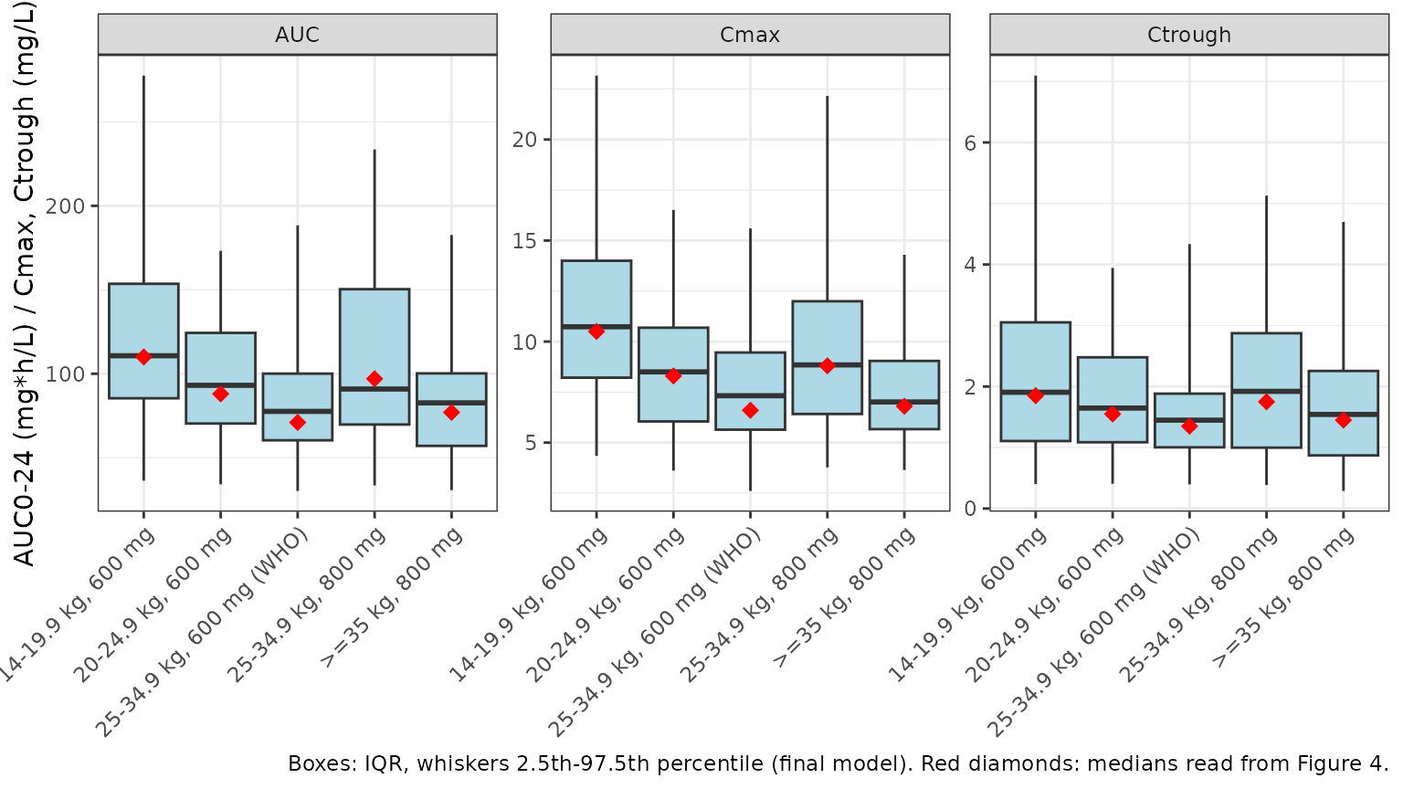
Replicates Figure 4 of Tsirizani 2024.
fig4_cmp <- expo |>
  dplyr::group_by(model, arm) |>
  dplyr::summarise(dplyr::across(c(AUC, Cmax, Ctrough), stats::median),
                   .groups = "drop") |>
  tidyr::pivot_longer(c(AUC, Cmax, Ctrough), names_to = "metric",
                      values_to = "simulated") |>
  dplyr::inner_join(fig4_long, by = c("arm", "metric")) |>
  dplyr::mutate(pct_diff = 100 * (simulated / value - 1))

fig4_cmp |>
  dplyr::mutate(arm = factor(arm, levels = arms$arm)) |>
  dplyr::arrange(model, metric, arm) |>
  dplyr::rename("Model" = model, "Arm" = arm, "Metric" = metric,
                "Simulated median" = simulated, "Figure 4 median" = value,
                "% difference" = pct_diff) |>
  knitr::kable(digits = 2,
caption = "Simulated cohort medians versus Figure 4 medians.")| Model | Arm | Metric | Simulated median | Figure 4 median | % difference |
|---|---|---|---|---|---|
| AAG binding (Supplementary Table 1) | 14-19.9 kg, 600 mg | AUC | 106.10 | 110.00 | -3.54 |
| AAG binding (Supplementary Table 1) | 20-24.9 kg, 600 mg | AUC | 95.02 | 88.00 | 7.98 |
| AAG binding (Supplementary Table 1) | 25-34.9 kg, 600 mg (WHO) | AUC | 78.78 | 71.00 | 10.95 |
| AAG binding (Supplementary Table 1) | 25-34.9 kg, 800 mg | AUC | 102.86 | 97.00 | 6.04 |
| AAG binding (Supplementary Table 1) | >=35 kg, 800 mg | AUC | 83.38 | 77.00 | 8.29 |
| AAG binding (Supplementary Table 1) | 14-19.9 kg, 600 mg | Cmax | 9.75 | 10.50 | -7.18 |
| AAG binding (Supplementary Table 1) | 20-24.9 kg, 600 mg | Cmax | 8.72 | 8.30 | 5.07 |
| AAG binding (Supplementary Table 1) | 25-34.9 kg, 600 mg (WHO) | Cmax | 7.14 | 6.60 | 8.15 |
| AAG binding (Supplementary Table 1) | 25-34.9 kg, 800 mg | Cmax | 9.68 | 8.80 | 9.97 |
| AAG binding (Supplementary Table 1) | >=35 kg, 800 mg | Cmax | 7.89 | 6.80 | 16.08 |
| AAG binding (Supplementary Table 1) | 14-19.9 kg, 600 mg | Ctrough | 1.69 | 1.85 | -8.73 |
| AAG binding (Supplementary Table 1) | 20-24.9 kg, 600 mg | Ctrough | 1.58 | 1.55 | 2.26 |
| AAG binding (Supplementary Table 1) | 25-34.9 kg, 600 mg (WHO) | Ctrough | 1.46 | 1.35 | 8.39 |
| AAG binding (Supplementary Table 1) | 25-34.9 kg, 800 mg | Ctrough | 2.09 | 1.75 | 19.70 |
| AAG binding (Supplementary Table 1) | >=35 kg, 800 mg | Ctrough | 1.56 | 1.45 | 7.63 |
| Final (Table 3) | 14-19.9 kg, 600 mg | AUC | 110.72 | 110.00 | 0.65 |
| Final (Table 3) | 20-24.9 kg, 600 mg | AUC | 93.11 | 88.00 | 5.80 |
| Final (Table 3) | 25-34.9 kg, 600 mg (WHO) | AUC | 77.59 | 71.00 | 9.28 |
| Final (Table 3) | 25-34.9 kg, 800 mg | AUC | 90.91 | 97.00 | -6.28 |
| Final (Table 3) | >=35 kg, 800 mg | AUC | 82.65 | 77.00 | 7.34 |
| Final (Table 3) | 14-19.9 kg, 600 mg | Cmax | 10.73 | 10.50 | 2.22 |
| Final (Table 3) | 20-24.9 kg, 600 mg | Cmax | 8.50 | 8.30 | 2.42 |
| Final (Table 3) | 25-34.9 kg, 600 mg (WHO) | Cmax | 7.32 | 6.60 | 10.92 |
| Final (Table 3) | 25-34.9 kg, 800 mg | Cmax | 8.85 | 8.80 | 0.51 |
| Final (Table 3) | >=35 kg, 800 mg | Cmax | 7.01 | 6.80 | 3.11 |
| Final (Table 3) | 14-19.9 kg, 600 mg | Ctrough | 1.91 | 1.85 | 3.02 |
| Final (Table 3) | 20-24.9 kg, 600 mg | Ctrough | 1.65 | 1.55 | 6.24 |
| Final (Table 3) | 25-34.9 kg, 600 mg (WHO) | Ctrough | 1.45 | 1.35 | 7.32 |
| Final (Table 3) | 25-34.9 kg, 800 mg | Ctrough | 1.92 | 1.75 | 9.76 |
| Final (Table 3) | >=35 kg, 800 mg | Ctrough | 1.54 | 1.45 | 6.40 |
final_auc <- dplyr::filter(fig4_cmp, model == "Final (Table 3)", metric == "AUC")
stopifnot(
  # The whole-cohort AUC centre: a mis-transcribed clearance or dose moves
  # every arm together by tens of percent.
  abs(stats::median(final_auc$pct_diff)) < 15,
  # Per-arm envelope, wide enough for 100-child cohort medians, the
  # within-band weight assumption and reading medians off a box plot.
  all(abs(final_auc$pct_diff) < 30)
)
The final model reproduces the Figure 4 pattern: the lightest band on 600 mg has the highest exposure, the WHO 600 mg dose in the 25-34.9 kg band gives the lowest, and the CHAPAS-4 800 mg dose in that band sits above the adult median AUC of 69.4 mg*h/L. The supplementary binding model gives similar total exposures.
PKNCA validation
PKNCA is run on the final-model cohort over the steady-state interval, using only the study’s sampling times (0, 1, 2, 4, 6, 8, 12 and 24 h), because the published NCA used those samples. Only the CHAPAS-4 arms are compared.
paper_times <- c(0, 1, 2, 4, 6, 8, 12, 24)
nca_conc <- sim |>
  dplyr::filter(!is.na(Cc), tad %in% paper_times,
                arm != "25-34.9 kg, 600 mg (WHO)") |>
  dplyr::select(id, band, tad, Cc)
nca_dose <- cohort |>
  dplyr::filter(arm != "25-34.9 kg, 600 mg (WHO)") |>
  dplyr::transmute(id, band, tad = 0, amt = dose)

conc_obj <- PKNCA::PKNCAconc(nca_conc, Cc ~ tad | band + id)
dose_obj <- PKNCA::PKNCAdose(nca_dose, amt ~ tad | band + id)
intervals <- data.frame(start = 0, end = 24, auclast = TRUE, cmax = TRUE,
                        cmin = TRUE)
nca_res <- PKNCA::pk.nca(PKNCA::PKNCAdata(conc_obj, dose_obj,
                                          intervals = intervals))
Comparison against published NCA
The paper’s NCA (Table 2, Supplementary Table 3) reports geometric
means of observed concentrations; the comparison table below reports
simulated medians, which for these log-normally distributed exposures
are close to geometric means. The trough is the 24 h concentration
(cmin over a steady-state interval).
published <- tibble::tribble(
  ~band,      ~auclast, ~cmax, ~cmin,
  "14-19.9",   98.5,     9.6,   1.4,
  "20-24.9",   94.7,     9.3,   1.3,
  "25-34.9",  100.4,     9.8,   1.7,
  ">=35",      82.3,     7.5,   1.8
)

cmp <- nlmixr2lib::ncaComparisonTable(
  simulated = nca_res,
  reference = published,
  by = "band",
  params = c("auclast", "cmax", "cmin"),
  units = c(auclast = "mg*h/L", cmax = "mg/L", cmin = "mg/L"),
  tolerance_pct = 20
)
knitr::kable(
  cmp,
  caption = paste("Simulated steady-state NCA (median) versus Supplementary",
                  "Table 3 geometric means by weight band.",
                  "* differs by more than 20%.")
)| NCA parameter | band | Reference | Simulated | % diff |
|---|---|---|---|---|
| Cmax (mg/L) | 14-19.9 | 9.6 | 10.6 | +10.1% |
| Cmax (mg/L) | 20-24.9 | 9.3 | 8.29 | -10.8% |
| Cmax (mg/L) | 25-34.9 | 9.8 | 8.43 | -14.0% |
| Cmax (mg/L) | >=35 | 7.5 | 6.91 | -7.9% |
| Cmin (mg/L) | 14-19.9 | 1.4 | 1.43 | +2.2% |
| Cmin (mg/L) | 20-24.9 | 1.3 | 1.4 | +8.0% |
| Cmin (mg/L) | 25-34.9 | 1.7 | 1.36 | -19.8% |
| Cmin (mg/L) | >=35 | 1.8 | 1.3 | -27.9%* |
| AUClast (mg*h/L) | 14-19.9 | 98.5 | 111 | +12.4% |
| AUClast (mg*h/L) | 20-24.9 | 94.7 | 93.8 | -1.0% |
| AUClast (mg*h/L) | 25-34.9 | 100 | 91.5 | -8.8% |
| AUClast (mg*h/L) | >=35 | 82.3 | 83.2 | +1.1% |
nca_auc <- as.data.frame(nca_res$result) |>
  dplyr::filter(PPTESTCD == "auclast")
pooled_gm <- exp(mean(log(nca_auc$PPORRES)))
c(simulated_pooled_GM_AUC = pooled_gm, Table2_GM_AUC = 94.3)
#> simulated_pooled_GM_AUC           Table2_GM_AUC
#>                93.14052                94.30000
stopifnot(abs(pooled_gm / 94.3 - 1) < 0.2)
The pooled geometric-mean AUC(0-24) agrees with the observed 94.3 mg*h/L of Table 2, and AUC and Cmax agree within 15% in every band. The trough in the heaviest band falls furthest from the observed value: the observed geometric mean is 1.8 mg/L in 13 children whose NCA half-life was unusually long and variable (13.4 h, 77% CV, Supplementary Table 3). The paper’s own Figure 4 simulation puts the median trough for that band near 1.45 mg/L, below the observed value too, so the gap is between the published model and that band’s observed data, not in the encoding.
Assumptions and deviations
-
Variability scale. Table 3 and Supplementary Table
1 give BSV and BOV as percentages without saying whether they are
log-scale standard deviations or coefficients of variation. The
maintainers read them as omega x 100 (omega^2 = (pct/100)^2), the
convention verified against the supplemental control stream of the same
group’s CHAPAS-4 ritonavir analysis
(
Tsirizani_2025_ritonavir). Reading them as CVs instead would shrink the 60.8% MTT BOV variance from 0.370 to 0.315. - Occasions. The paper says only that BOV was placed on the absorption parameters. Each child had one intensive PK day, so the occasions are taken to be the unwitnessed doses before the PK day (OCC = 1) and the witnessed PK-day dose (OCC = 2), as in the ritonavir analysis, with one shared variance per parameter. The 2.14-fold BOV inflation estimated for unwitnessed ritonavir doses is not part of this darunavir model.
-
Transit chain. The paper cites Savic 2007 for the
transit compartments; the model uses that parameterisation,
ktr = (NN + 1) / MTT, with the chain feeding an absorption compartment drained atka(Supplementary Figure 2). The non-integer NN is implemented with the closed-form gamma input, which is exact for daily dosing because the chain empties within a few hours. - AAG reference. The clearance equation centres AAG at 0.66 g/L (Table 3 footnote c) while the binding model centres Bmax at 0.7 g/L (Supplementary Table 1 footnote), the rounded Table 1 median. Both are used as printed.
-
Binding-model structure. Supplementary Figure 2
shows free darunavir exchanging with the peripheral compartment and
being cleared; the model therefore treats the peripheral compartment as
holding free drug, with central-to-peripheral flux
Q * Cfreeand return fluxQ * Aperipheral / Vp. Binding is instantaneous and solved in closed form from the total concentration. Several binding-model parameters (CLint, Q, V2, NN, Kd, Bmax) are printed without a confidence interval; the Discussion states they were estimated with priors from Schalkwijk et al., so they are not marked as fixed. - Virtual cohort. Weight is uniform within each band and AAG log-normal (median 0.7 g/L, log-SD 0.35, clamped to 0.3-1.9 g/L); the paper’s 100,000-child simulation population is not described further. The Figure 1 and Figure 4 medians were read from the published images by the maintainers and are approximate.
- NRTI backbone, age and ritonavir exposure had no significant effect and are not in either model.
- No correction notice for the article was found in Europe PMC as of 2026-10-31.