Morphine (Franken 2015)
Source:vignettes/articles/Franken_2015_morphine.Rmd
Franken_2015_morphine.RmdModel and source
- Citation: Franken LG, Masman AD, de Winter BCM, Koch BCP, Baar FPM, Tibboel D, van Gelder T, Mathot RAA. Pharmacokinetics of Morphine, Morphine-3-Glucuronide and Morphine-6-Glucuronide in Terminally Ill Adult Patients. Clin Pharmacokinet. 2016;55(6):697-709 (published online 29 December 2015). doi:10.1007/s40262-015-0345-4.
- Description: Joint parent-metabolite population PK model for morphine and its two glucuronide metabolites (M3G, M6G) in 47 terminally ill adult palliative care patients (Franken 2015). Morphine: two-compartment disposition with three parallel first-order absorption routes (subcutaneous bolus, immediate-release oral liquid, controlled-release oral tablet) using route-specific fixed absorption rate constants; oral bioavailability F is estimated (SC F assumed 1). M3G and M6G are each one-compartment models fed by fixed-fraction transformation of morphine clearance (Fm1 = 0.55 for M3G, Fm2 = 0.10 for M6G, both fixed from literature). Morphine clearance decreases exponentially as time-to-death (TTD, days) approaches zero. Metabolite clearance depends on estimated glomerular filtration rate (eGFR, MDRD four-variable formula) and serum albumin via shared power-form covariate exponents. Residual variability was reported as additive error on the log-transformed observation (LTBS).
- Article: https://doi.org/10.1007/s40262-015-0345-4
Population
The published analysis included 47 terminally ill adult
palliative-care patients admitted to the Laurens Cadenza hospice in
Rotterdam over a 2-year period. Median age 71 years (range 43-93), 55.3%
female, 95.7% Caucasian and 4.3% Afro-Caribbean, with 95.7% having
advanced malignancy as the primary diagnosis. Median duration of
admittance was 33 days (range 7-457). Patients received morphine for
pain and dyspnoea at daily doses of 15-540 mg administered as oral
controlled-release tablets, oral immediate-release liquid, or
subcutaneous bolus / infusion. Sparse plasma sampling (median 2 samples
per subject, range 1-10) yielded 152 plasma concentrations for morphine,
M3G, and M6G. Baseline blood chemistry medians at admission included
albumin 26 g/L (range 14-39), creatinine 72 umol/L, and eGFR
(four-variable MDRD) 96 mL/min/1.73 m^2 (range 27-239). See Franken 2015
Table 1 for the full baseline summary; the same information is available
programmatically via
readModelDb("Franken_2015_morphine")$population.
Source trace
The per-parameter origin is recorded as an in-file comment next to
each ini() entry in
inst/modeldb/specificDrugs/Franken_2015_morphine.R. The
table below collects them in one place.
| Equation / parameter | Final value | Source location |
|---|---|---|
lka_sc (Ka SC bolus) |
10 1/h (FIXED) | Methods 3.1 (literature [26, 27]) |
lka_oral_ir (Ka IR liquid) |
6 1/h (FIXED) | Methods 3.1 (literature [26, 27]) |
lka_oral_cr (Ka CR tablet) |
0.8 1/h (FIXED) | Methods 3.1 (literature [26, 27]) |
lfdepot (F oral) |
0.30 | Table 2 Final |
lcl (morphine CL asymptote) |
47.5 L/h | Table 2 Final |
lvc (V1) |
190 L | Table 2 Final |
lq (Q) |
76.1 L/h | Table 2 Final |
lvp (V2) |
243 L | Table 2 Final |
lcl_m3g (CL M3G) |
1.44 L/h | Table 2 Final |
lvc_m3g (V M3G) |
8.02 L | Table 2 Final |
lcl_m6g (CL M6G) |
1.78 L/h | Table 2 Final |
lvc_m6g (V M6G) |
8.24 L | Table 2 Final |
fm_m3g (Fm1) |
0.55 (FIXED) | Methods 2.3.1 (literature [21-23]) |
fm_m6g (Fm2) |
0.10 (FIXED) | Methods 2.3.1 (literature [21-23]) |
ttd_d (TTD peak drop in CL) |
17.6 L/h | Table 2 Final |
ttd_rate (TTD first-order rate) |
0.13 1/day | Table 2 Final |
e_crcl_cl_m3g = e_crcl_cl_m6g (eGFR
exponent) |
0.673 | Table 2 Final (shared coefficient) |
e_alb_cl_m3g = e_alb_cl_m6g (albumin
exponent) |
1.1 | Table 2 Final (shared coefficient) |
etalfdepot (BSV on F) |
37.8% CV | Table 2 Final |
etalcl (BSV on morphine CL) |
53.4% CV | Table 2 Final |
etalcl_m3g, etalcl_m6g
|
29.3% / 34.3% CV, rho = 1 | Table 2 Final + Section 3.1 |
etalvc_m3g, etalvc_m6g
|
151.7% / 143.0% CV, rho = 1 | Table 2 Final + Section 3.1 |
expSd (morphine residual) |
sqrt(0.432) | Table 2 Final (LTBS variance) |
expSd_m3g (M3G residual) |
sqrt(0.246) | Table 2 Final (LTBS variance) |
expSd_m6g (M6G residual) |
sqrt(0.265) | Table 2 Final (LTBS variance) |
| Equation: morphine 2-cmt model with three parallel depots | n/a | Figure 2 schematic |
| Equation: TTD covariate first-order decay on CL | n/a | Eq. 3, Section 2.3.2 |
| Equation: eGFR / albumin power covariates on metabolite CL | n/a | Eq. 1, Section 2.3.2 |
Virtual cohort
Original observed concentrations are not publicly available. The simulations below use typical-value virtual subjects whose covariates approximate the representative scenarios shown in Franken 2015 Figures 3-5. The model is exercised at the four eGFR levels of Figure 3, the three albumin levels of Figure 4, and the three time-before-death scenarios of Figure 5.
set.seed(20151229)

# Figure 3 cohort: vary eGFR at constant albumin = 25 g/L, TTD large
fig3 <- data.frame(
  id    = 1:4,
  CRCL  = c(10, 30, 50, 90),
  ALB   = 25,
  TTD   = 100,                       # "far from death" baseline
  scenario = factor(
    paste0("eGFR ", c(10, 30, 50, 90), " mL/min"),
    levels = paste0("eGFR ", c(10, 30, 50, 90), " mL/min")
  ),
  stringsAsFactors = FALSE
)

# Figure 4 cohort: vary albumin at eGFR = 78 mL/min, TTD large
fig4 <- data.frame(
  id    = 5:7,
  CRCL  = 78,
  ALB   = c(15, 25, 35),
  TTD   = 100,
  scenario = factor(
    paste0("albumin ", c(15, 25, 35), " g/L"),
    levels = paste0("albumin ", c(15, 25, 35), " g/L")
  ),
  stringsAsFactors = FALSE
)

# Figure 5 cohort: vary TTD at fixed eGFR / albumin (population medians)
fig5 <- data.frame(
  id    = 8:10,
  CRCL  = 96,
  ALB   = 26,
  TTD   = c(14, 7, 1),               # 2 weeks, 1 week, 1 day before death
  scenario = factor(
    paste0(c("2 wk", "1 wk", "1 day"), " before death"),
    levels = paste0(c("2 wk", "1 wk", "1 day"), " before death")
  ),
  stringsAsFactors = FALSE
)
Simulation
Figures 3 and 4 use a 30 mg subcutaneous bolus six times daily for
ten days; Figure 5 uses a 50 mg subcutaneous bolus six times daily over
the final week of life. Subcutaneous bioavailability is structurally 1
(so the SC depot’s f defaults to 1); oral routes (depot2 =
IR liquid, depot3 = CR tablet) carry the estimated f_oral.
All simulations use typical-value parameters
(rxode2::zeroRe()) so the plots are mean-curve replications
of the published figures rather than VPCs.
mod_typical <- readModelDb("Franken_2015_morphine") |> rxode2::zeroRe()

build_events <- function(cov_df, obs_times, dose_events) {
  events_list <- lapply(seq_len(nrow(cov_df)), function(i) {
    row <- cov_df[i, , drop = FALSE]
    dose_rows <- dose_events |>
      mutate(
        id       = row$id,
        CRCL     = row$CRCL,
        ALB      = row$ALB,
        TTD      = row$TTD,
        scenario = as.character(row$scenario)
      )
    obs_rows <- data.frame(
      id       = row$id,
      time     = obs_times,
      amt      = NA_real_,
      rate     = NA_real_,
      evid     = 0L,
      cmt      = "Cc",
      CRCL     = row$CRCL,
      ALB      = row$ALB,
      TTD      = row$TTD,
      scenario = as.character(row$scenario),
      stringsAsFactors = FALSE
    )
    dplyr::bind_rows(dose_rows, obs_rows)
  })
  dplyr::bind_rows(events_list) |>
    arrange(id, time, evid)
}

# 30 mg SC q4h x 10 days for Figures 3 and 4 (240 h total observation window)
dose_30mg_q4h <- data.frame(
  time = seq(0, 240 - 4, by = 4),
  amt  = 30,
  rate = 0,
  evid = 1L,
  cmt  = "depot",                    # SC bolus -> depot (depot1)
  stringsAsFactors = FALSE
)

obs_times_240 <- c(seq(0, 24, by = 0.25), seq(25, 240, by = 1))

events_fig3 <- build_events(fig3, obs_times_240, dose_30mg_q4h)
events_fig4 <- build_events(fig4, obs_times_240, dose_30mg_q4h)

sim_fig3 <- rxode2::rxSolve(
  mod_typical, events = events_fig3,
  keep = c("scenario", "CRCL", "ALB", "TTD")
) |> as.data.frame()
#> ℹ omega/sigma items treated as zero: 'etalfdepot', 'etalcl', 'etalcl_m3g', 'etalcl_m6g', 'etalvc_m3g', 'etalvc_m6g'
#> Warning: multi-subject simulation without without 'omega'
sim_fig4 <- rxode2::rxSolve(
  mod_typical, events = events_fig4,
  keep = c("scenario", "CRCL", "ALB", "TTD")
) |> as.data.frame()
#> ℹ omega/sigma items treated as zero: 'etalfdepot', 'etalcl', 'etalcl_m3g', 'etalcl_m6g', 'etalvc_m3g', 'etalvc_m6g'
#> Warning: multi-subject simulation without without 'omega'

# 50 mg SC q4h x 24 h for Figure 5 (TTD effect)
dose_50mg_q4h <- data.frame(
  time = seq(0, 24 - 4, by = 4),
  amt  = 50,
  rate = 0,
  evid = 1L,
  cmt  = "depot",
  stringsAsFactors = FALSE
)
obs_times_24 <- c(seq(0, 4, by = 0.1), seq(4.5, 24, by = 0.5))

events_fig5 <- build_events(fig5, obs_times_24, dose_50mg_q4h)
sim_fig5 <- rxode2::rxSolve(
  mod_typical, events = events_fig5,
  keep = c("scenario", "CRCL", "ALB", "TTD")
) |> as.data.frame()
#> ℹ omega/sigma items treated as zero: 'etalfdepot', 'etalcl', 'etalcl_m3g', 'etalcl_m6g', 'etalvc_m3g', 'etalvc_m6g'
#> Warning: multi-subject simulation without without 'omega'
Replicate published figures
Figure 3: effect of eGFR on M3G / M6G concentrations
plot_fig3 <- sim_fig3 |>
  pivot_longer(cols = c(Cc, Cc_m3g, Cc_m6g),
               names_to = "species", values_to = "conc") |>
  mutate(species = factor(
    recode(species,
           "Cc"     = "Morphine",
           "Cc_m3g" = "M3G",
           "Cc_m6g" = "M6G"),
    levels = c("Morphine", "M3G", "M6G")
  ))

ggplot(plot_fig3, aes(x = time, y = conc, color = scenario)) +
  geom_line(linewidth = 0.8) +
  facet_wrap(~species, scales = "free_y", ncol = 3) +
  labs(x = "Time (h)",
       y = "Concentration (ug/L; morphine equivalents)",
       color = "eGFR scenario",
       title = "Replicates Figure 3 of Franken 2015",
       caption = paste("30 mg subcutaneous morphine every 4 h x 10 days,",
                       "albumin held at 25 g/L, TTD = 100 days.",
                       "Typical-value simulation (no IIV / no RUV)."))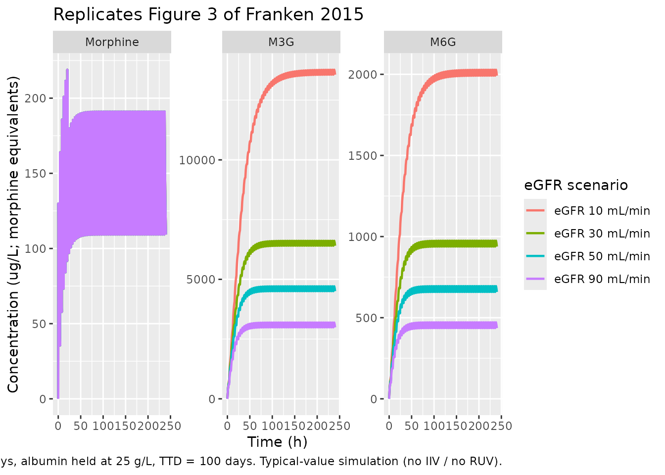
Figure 4: effect of serum albumin on M3G / M6G concentrations
plot_fig4 <- sim_fig4 |>
  pivot_longer(cols = c(Cc, Cc_m3g, Cc_m6g),
               names_to = "species", values_to = "conc") |>
  mutate(species = factor(
    recode(species,
           "Cc"     = "Morphine",
           "Cc_m3g" = "M3G",
           "Cc_m6g" = "M6G"),
    levels = c("Morphine", "M3G", "M6G")
  ))

ggplot(plot_fig4, aes(x = time, y = conc, color = scenario)) +
  geom_line(linewidth = 0.8) +
  facet_wrap(~species, scales = "free_y", ncol = 3) +
  labs(x = "Time (h)",
       y = "Concentration (ug/L; morphine equivalents)",
       color = "Albumin scenario",
       title = "Replicates Figure 4 of Franken 2015",
       caption = paste("30 mg subcutaneous morphine every 4 h x 10 days,",
                       "eGFR held at 78 mL/min/1.73 m^2, TTD = 100 days.",
                       "Typical-value simulation."))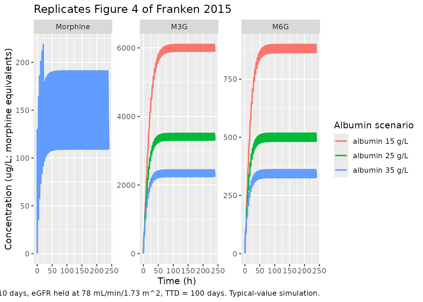
Figure 5: effect of time-to-death on morphine concentrations
plot_fig5 <- sim_fig5 |>
  filter(time > 0)

ggplot(plot_fig5, aes(x = time, y = Cc, color = scenario)) +
  geom_line(linewidth = 0.8) +
  labs(x = "Time after first dose (h)",
       y = "Morphine concentration (ug/L)",
       color = "Time before death",
       title = "Replicates Figure 5 of Franken 2015",
       caption = paste("50 mg subcutaneous morphine every 4 h x 24 h,",
                       "eGFR and albumin held at population medians.",
                       "Typical-value simulation (no IIV / no RUV)."))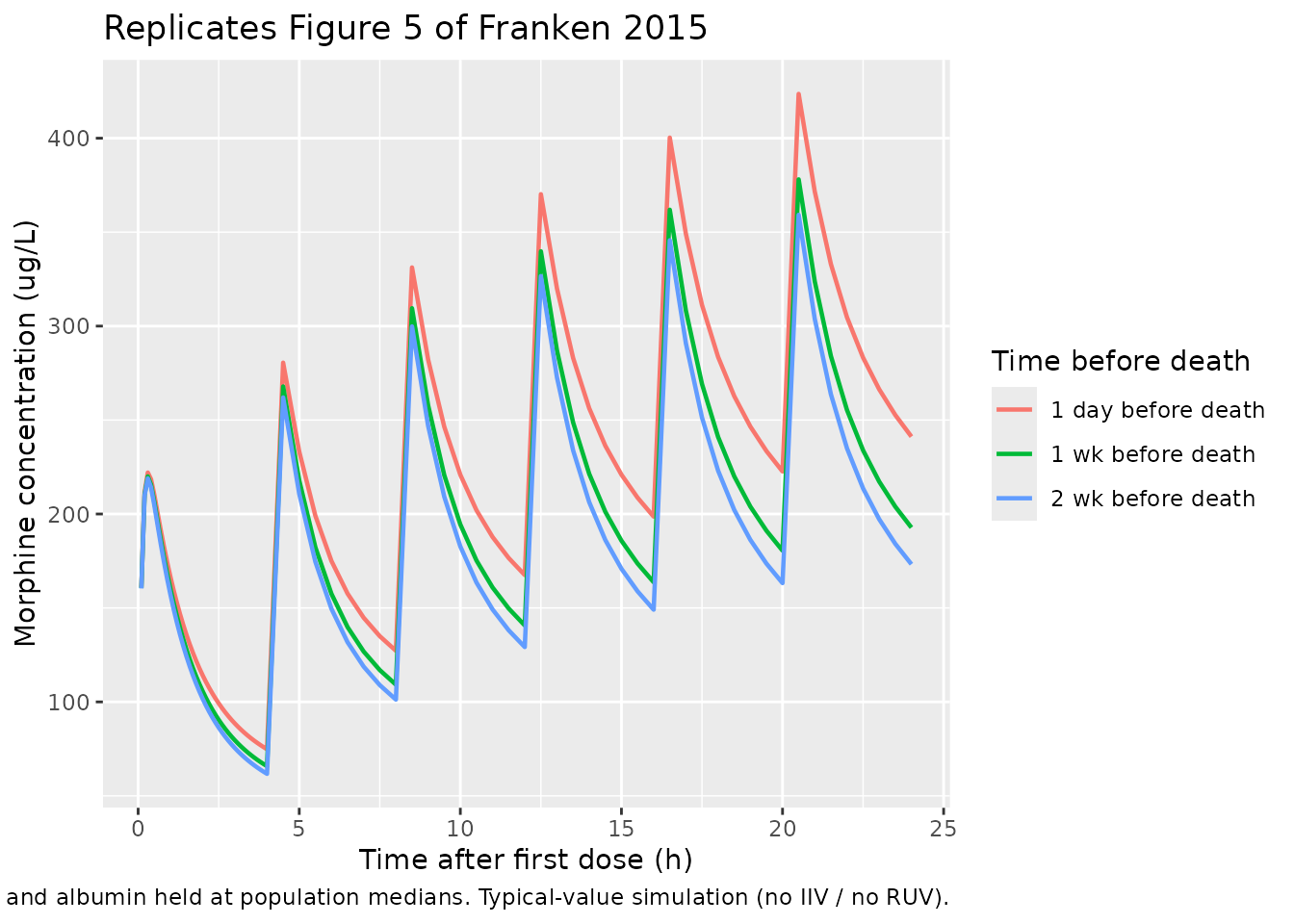
Numeric checks against Section 3.3
Franken 2015 Section 3.3 quotes three numeric results from the final-model simulations:
-
Morphine CL declines with TTD. Paper: 46.4 L/h
three weeks before death (TTD = 21 d), 40.6 L/h one week before death
(TTD = 7 d), and 29.9 L/h on the day of death (TTD = 0 d). The model
encodes
CL(TTD) = 47.5 - 17.6 * exp(-0.13 * TTD).
ttd_grid <- data.frame(TTD = c(21, 7, 0)) |>
  mutate(CL_predicted = 47.5 - 17.6 * exp(-0.13 * TTD),
         CL_paper     = c(46.4, 40.6, 29.9))
knitr::kable(ttd_grid, caption = "Morphine CL by TTD: predicted vs published Section 3.3.")| TTD | CL_predicted | CL_paper |
|---|---|---|
| 21 | 46.35214 | 46.4 |
| 7 | 40.41557 | 40.6 |
| 0 | 29.90000 | 29.9 |
- M3G CL decline with eGFR. Paper: at albumin = 25 g/L, M3G CL drops from ~1.6 L/h at eGFR = 90 mL/min to ~1.1 L/h at eGFR = 50 mL/min (~30% reduction). The packaged model uses references CRCL_ref = 96 (the Table 1 admission-time population median) and ALB_ref = 26, so the absolute typical-value M3G CL differs slightly from the paper’s narrative; the relative drop matches.
m3g_grid <- data.frame(CRCL = c(90, 50, 30, 10), ALB = 25) |>
  mutate(CL_m3g_predicted = 1.44 * (CRCL / 96)^0.673 * (ALB / 26)^1.1)
knitr::kable(m3g_grid, caption = "Typical-value M3G CL across eGFR at albumin = 25 g/L.")| CRCL | ALB | CL_m3g_predicted |
|---|---|---|
| 90 | 25 | 1.3205732 |
| 50 | 25 | 0.8891276 |
| 30 | 25 | 0.6304634 |
| 10 | 25 | 0.3009936 |
- M3G CL decline with albumin. Paper: at eGFR = 78 mL/min, M3G CL drops from ~2.1 L/h at albumin = 35 g/L to ~1.4 L/h at albumin = 25 g/L (~31% reduction).
alb_grid <- data.frame(ALB = c(35, 25, 15), CRCL = 78) |>
  mutate(CL_m3g_predicted = 1.44 * (CRCL / 96)^0.673 * (ALB / 26)^1.1)
knitr::kable(alb_grid, caption = "Typical-value M3G CL across albumin at eGFR = 78 mL/min.")| ALB | CRCL | CL_m3g_predicted |
|---|---|---|
| 35 | 78 | 1.7365120 |
| 25 | 78 | 1.1993252 |
| 15 | 78 | 0.6837594 |
PKNCA validation
Single-dose NCA after the first 30 mg subcutaneous bolus of the Figure 3 cohort (window 0-4 h, before the second dose), computed separately for morphine and each metabolite. Treatment grouping uses the four eGFR scenarios so per-group summaries roll up.
sim_nca_window <- sim_fig3 |> filter(time <= 4)

dose_df_fig3 <- events_fig3 |>
  filter(evid == 1L, time == 0) |>
  select(id, time, amt, scenario)

intervals_sd <- data.frame(
  start    = 0,
  end      = 4,
  cmax     = TRUE,
  tmax     = TRUE,
  auclast  = TRUE,
  half.life = FALSE
)
Morphine
sim_nca_morphine <- sim_nca_window |>
  filter(!is.na(Cc)) |>
  select(id, time, Cc, scenario)

conc_obj_morphine <- PKNCA::PKNCAconc(
  sim_nca_morphine, Cc ~ time | scenario + id,
  concu = "ug/L", timeu = "h"
)
dose_obj <- PKNCA::PKNCAdose(
  dose_df_fig3, amt ~ time | scenario + id, doseu = "mg"
)

nca_morphine <- PKNCA::pk.nca(
  PKNCA::PKNCAdata(conc_obj_morphine, dose_obj, intervals = intervals_sd)
)
knitr::kable(as.data.frame(summary(nca_morphine)),
caption = "Morphine NCA over the 4 h after the first 30 mg SC bolus.")| Interval Start | Interval End | scenario | N | AUClast (h*ug/L) | Cmax (ug/L) | Tmax (h) |
|---|---|---|---|---|---|---|
| 0 | 4 | eGFR 10 mL/min | 1 | 265 | 130 | 0.250 |
| 0 | 4 | eGFR 30 mL/min | 1 | 265 | 130 | 0.250 |
| 0 | 4 | eGFR 50 mL/min | 1 | 265 | 130 | 0.250 |
| 0 | 4 | eGFR 90 mL/min | 1 | 265 | 130 | 0.250 |
M3G
sim_nca_m3g <- sim_nca_window |>
  filter(!is.na(Cc_m3g)) |>
  select(id, time, Cc_m3g, scenario) |>
  rename(Cc = Cc_m3g)

conc_obj_m3g <- PKNCA::PKNCAconc(
  sim_nca_m3g, Cc ~ time | scenario + id,
  concu = "ug/L", timeu = "h"
)
nca_m3g <- PKNCA::pk.nca(
  PKNCA::PKNCAdata(conc_obj_m3g, dose_obj, intervals = intervals_sd)
)
knitr::kable(as.data.frame(summary(nca_m3g)),
caption = "M3G NCA over the 4 h after the first 30 mg SC morphine bolus.")| Interval Start | Interval End | scenario | N | AUClast (h*ug/L) | Cmax (ug/L) | Tmax (h) |
|---|---|---|---|---|---|---|
| 0 | 4 | eGFR 10 mL/min | 1 | 2060 | 812 | 4.00 |
| 0 | 4 | eGFR 30 mL/min | 1 | 1940 | 737 | 4.00 |
| 0 | 4 | eGFR 50 mL/min | 1 | 1860 | 683 | 4.00 |
| 0 | 4 | eGFR 90 mL/min | 1 | 1730 | 605 | 4.00 |
M6G
sim_nca_m6g <- sim_nca_window |>
  filter(!is.na(Cc_m6g)) |>
  select(id, time, Cc_m6g, scenario) |>
  rename(Cc = Cc_m6g)

conc_obj_m6g <- PKNCA::PKNCAconc(
  sim_nca_m6g, Cc ~ time | scenario + id,
  concu = "ug/L", timeu = "h"
)
nca_m6g <- PKNCA::pk.nca(
  PKNCA::PKNCAdata(conc_obj_m6g, dose_obj, intervals = intervals_sd)
)
knitr::kable(as.data.frame(summary(nca_m6g)),
caption = "M6G NCA over the 4 h after the first 30 mg SC morphine bolus.")| Interval Start | Interval End | scenario | N | AUClast (h*ug/L) | Cmax (ug/L) | Tmax (h) |
|---|---|---|---|---|---|---|
| 0 | 4 | eGFR 10 mL/min | 1 | 360 | 141 | 4.00 |
| 0 | 4 | eGFR 30 mL/min | 1 | 336 | 126 | 4.00 |
| 0 | 4 | eGFR 50 mL/min | 1 | 318 | 115 | 4.00 |
| 0 | 4 | eGFR 90 mL/min | 1 | 292 | 99.4 | 4.00 |
Assumptions and deviations
-
Residual-error interpretation. Franken 2015 Methods
2.3.1 reports residual variability as “additive error on the log scale”
with Table 2 Final values 0.432 (morphine), 0.246 (M3G), 0.265 (M6G), no
explicit units. The packaged model interprets these as NONMEM
$SIGMAvariance estimates on the log scale and supplies their square roots to rxode2’slnorm()residual model so thatlog(Cobs) - log(Cpred) ~ N(0, expSd^2). If a future reading determines the values were already reported as log-scale SDs, theexpSd*parameters should be set equal to the published numbers (without the square root). - Covariate reference values. The paper Methods 2.3.2 states “Continuous covariates were normalised to the population median values” without explicitly tabulating those medians per model. The packaged model uses the Table 1 admission medians eGFR = 96 mL/min/1.73 m^2 and albumin = 26 g/L as the reference. Section 3.3 simulation narratives imply a slightly different effective reference (the typical-value M3G CL at eGFR = 90 / albumin = 25 quoted as ~1.6 L/h is ~20% higher than the model evaluated at those covariates with admission-median references); this may reflect using the across-time median in the modeling dataset rather than the admission median in Table 1, but the exact reference is not stated. The relative effects of eGFR and albumin on metabolite CL match the paper’s reported ratios closely.
-
Shared covariate exponents on M3G and M6G
clearance. Table 2’s “Covariate effect on M3G and M6G
clearance” row reports a single eGFR coefficient (0.673) and a single
albumin coefficient (1.1) applied to both metabolite clearances. The
packaged model duplicates the coefficient onto the metabolite-suffixed
names (
e_crcl_cl_m3g=e_crcl_cl_m6g= 0.673;e_alb_cl_m3g=e_alb_cl_m6g= 1.1) so that the source-trace is explicit at the metabolite level. The nlmixr2lib convention does not currently have a syntactic form for “single estimate shared across metabolite suffixes”, so the duplication is the cleanest available encoding. - Fixed transformation fractions Fm1 = 0.55, Fm2 = 0.10. Per Methods 2.3.1, the fractions of morphine clearance that produce M3G and M6G could not be identified from the data (no mass-balance / urine measurements) and were fixed to literature values [21-23]. The metabolite clearance and metabolite volume estimates are therefore apparent values proportional to the assumed fractions; refitting under different Fm1 / Fm2 values would rescale CL_M3G and V_M3G (and similarly for M6G) by the same factor.
-
Three parallel depots for the three administration
routes. The paper used route-specific fixed absorption rate
constants (10 1/h SC, 6 1/h oral IR, 0.8 1/h oral CR) with a single
estimated oral bioavailability F = 0.30 and an assumed SC
bioavailability of 1. The packaged model encodes this as three parallel
depot compartments (
depot,depot2,depot3for SC, oral IR, and oral CR respectively), withf(depot2)andf(depot3)set to the estimatedf_oraland SC using the rxode2 default of 1. A dosing record selects the route by itscmtvalue. -
TTD covariate is retrospective. The paper’s TTD
covariate is the number of days remaining until the patient’s recorded
time of death, which is known only after the fact. For prospective
simulation of virtual cohorts where time of death is not known, set
TTDto a large value (> 50 days) to recover the asymptotic typical-value morphine CL of 47.5 L/h. The packaged virtual cohorts in Figures 3-4 useTTD = 100days for this purpose; Figure 5 deliberately varies TTD. - Dose unit is mg of morphine free base. The paper expressed M3G and M6G concentrations “in their morphine equivalents using the molecular weight” (Methods 2.3.1), so all internal state quantities are tracked in mg of morphine-equivalents and the observation equations convert mg/L to ug/L by a factor of 1000.
-
eGFR (CRCL canonical name). The paper used the
four-variable Modification of Diet in Renal Disease (MDRD) formula; the
canonical covariate
CRCLregister name covers MDRD-derived eGFR with the source aliaseGFR. ThecovariateData[[CRCL]]$source_namefield records the alias.