Fondaparinux (Zufferey 2018)
Source:vignettes/articles/Zufferey_2018_fondaparinux.Rmd
Zufferey_2018_fondaparinux.RmdModel and source
- Citation: Zufferey PJ, Ollier E, Delavenne X, Laporte S, Mismetti P, Duffull SB. Incidence and risk factors of major bleeding following major orthopaedic surgery with fondaparinux thromboprophylaxis. A time-to-event analysis. Br J Clin Pharmacol. 2018;84(10):2242-2251. doi:10.1111/bcp.13663.
- Description: Parametric time-to-event model for major bleeding after major orthopaedic surgery under fondaparinux thromboprophylaxis (POP-A-RIX 2.5 mg once daily and PROPICE 1.5 mg once daily pooled cohorts; n = 1393, 64 adjudicated bleeding events). The hazard is hz(t) = h0(t) * exp(beta1SEX + beta2AUCinf/8.5 + beta3LBM/44), with gamma-shaped baseline h0(t) = theta1theta2(t-theta3)exp(-theta2(t-theta3)) for t > theta3 and 0 otherwise (lag time theta3 ~= 17.6 h, peak ~4 days post-surgery). AUCinf is derived inside the model from daily dose and clearance using the paper’s PK equation CL = 0.34 (CRCL/60)^0.485 * exp(eta) (lean-body-weight Cockcroft-Gault CrCl).
- Article: https://doi.org/10.1111/bcp.13663
This vignette validates the parametric time-to-event (TTE) model
packaged at
inst/modeldb/specificDrugs/Zufferey_2018_fondaparinux.R.
The model predicts the probability of major bleeding during fondaparinux
thromboprophylaxis after major orthopaedic surgery; clearance is
computed from Cockcroft-Gault creatinine clearance with lean body weight
(CrCl_LBW), AUCinf is derived as daily-dose / CL, and the hazard depends
on sex, AUCinf, and lean body mass.
Population
The pooled cohort combines two French multicentre prospective open-label studies in adults undergoing major orthopaedic surgery (hip arthroplasty, knee arthroplasty, or hip fracture surgery):
- POP-A-RIX (n = 957; ClinicalTrials.gov NCT01063543) – subjects with preoperative CrCl > 30 mL/min, treated with fondaparinux 2.5 mg subcutaneously once daily.
- PROPICE (n = 436; NCT00555438) – subjects with moderate renal impairment (CrCl 20-50 mL/min by Cockcroft-Gault), treated with fondaparinux 1.5 mg SC once daily.
Pooled baseline characteristics (Zufferey 2018 Table 1): n = 1393, mean age 76 +/- 11 years (range 24-101), mean body weight 68 +/- 16 kg (35-172), mean lean body weight 44 +/- 10 kg (26-93), mean CrCl_LBW 41 +/- 20 mL/min (10-173), 74% female. Surgical mix: 38% hip arthroplasty, 27% knee arthroplasty, 35% hip fracture. Sixty-four adjudicated major bleedings were observed (5.2% by day 11; Table 2).
The population metadata is available programmatically:
m <- readModelDb("Zufferey_2018_fondaparinux")
str(m()$meta$population, max.level = 1)
#> List of 13
#>  $ species       : chr "human"
#>  $ n_subjects    : int 1393
#>  $ n_studies     : int 2
#>  $ age_range     : chr "24-101 years (mean 76)"
#>  $ age_median    : chr "76 years"
#>  $ weight_range  : chr "35-172 kg (mean 68)"
#>  $ weight_median : chr "68 kg"
#>  $ sex_female_pct: num 74
#>  $ race_ethnicity: NULL
#>  $ disease_state : chr "Adults undergoing major orthopaedic surgery (primary or revision hip arthroplasty, primary or revision knee art"| __truncated__
#>  $ dose_range    : chr "1.5 mg or 2.5 mg subcutaneously once daily, first dose at least 6 h postoperatively; recommended thromboprophyl"| __truncated__
#>  $ regions       : chr "France (two multicentre prospective open-label cohorts)"
#>  $ notes         : chr "64 adjudicated major-bleeding events (4.6% of pooled cohort; 5.2% by day 11). LBM mean 44 kg (range 26-93). Coc"| __truncated__
Source trace
The per-parameter origin is captured as in-file comments next to each
ini() entry in
inst/modeldb/specificDrugs/Zufferey_2018_fondaparinux.R.
The table below collects them in one place.
| Equation / parameter | Value | Source location |
|---|---|---|
| CL = 0.34 * (CrCl_LBW/60)^0.485 * exp(b) | n/a | Page 5 (clearance equation, simulation section) |
lcl (log typical CL, L/h) |
log(0.34) | Page 5 CL equation: TVCL = 0.34 L/h |
e_crcl_cl (CRCL power exponent) |
0.485 | Page 5 CL equation |
etalcl (CV% = 34 on CL) |
0.10936 | Page 5: “log normal between subject variability of 34 (CV%)” |
base_haz1 (theta1, 1/h) |
0.00122 | Table 3, Full hazard model row theta1; bootstrap 95% CI 2e-5 to 2.4e-3 |
base_haz2 (theta2, 1/h) |
0.0122 | Table 3, Full hazard model row theta2; bootstrap 95% CI 0.0086-0.0158 |
t_lag (theta3, h) |
17.6 | Table 3, Full hazard model row theta3; bootstrap 95% CI 9.23-25.9 |
e_sexf_bleed (beta1, sex effect) |
1.62 | Table 3, beta1 * SEX; HR for males = exp(1.62) = 5.05 |
e_auc_bleed (beta2, AUC effect) |
0.975 | Table 3, beta2 * AUCinf/8.5 |
e_lbm_bleed (beta3, LBM effect) |
-1.93 | Table 3, beta3 * LBW/44; LBM increase reduces hazard |
| Hazard h0(t) gamma form (lag, peak ~day 4) | n/a | Derived by differentiating page 7 Hz(t) closed form; Figure 2 confirms shape |
| AUCinf reference 8.5 mg*h/L | – | Table 1 pooled-cohort mean AUCinf |
| LBW reference 44 kg | – | Table 1 pooled-cohort mean LBW |
Virtual cohort
The original POP-A-RIX and PROPICE per-subject data are not publicly available. We construct two virtual cohorts whose marginal distributions of CrCl_LBW, LBM, and sex approximate the pooled-cohort baseline characteristics (Table 1):
set.seed(20260526)

make_cohort <- function(n, dose_mg, crcl_mean, crcl_sd, crcl_lo, crcl_hi,
                        id_offset = 0L) {
  tibble(
    id    = id_offset + seq_len(n),
    SEXF  = as.integer(runif(n) < 0.74),
    LBM   = pmax(26, pmin(93, round(ifelse(SEXF == 1L,
                                           rnorm(n, mean = 42, sd = 9),
                                           rnorm(n, mean = 55, sd = 10)), 1))),
    CRCL  = pmax(crcl_lo, pmin(crcl_hi,
                               round(rnorm(n, mean = crcl_mean, sd = crcl_sd), 1))),
    DOSE  = dose_mg
  )
}

# POP-A-RIX: CrCl > 30 (LBW-Cockcroft mean 48, range 13-173) on 2.5 mg
poparix  <- make_cohort(n = 600, dose_mg = 2.5,
                        crcl_mean = 48, crcl_sd = 20, crcl_lo = 15, crcl_hi = 173,
                        id_offset = 0L)
# PROPICE: moderate renal impairment (LBW-Cockcroft mean 27, range 10-44) on 1.5 mg
propice  <- make_cohort(n = 400, dose_mg = 1.5,
                        crcl_mean = 27, crcl_sd = 7, crcl_lo = 10, crcl_hi = 44,
                        id_offset = 600L)

cohort_subjects <- bind_rows(
  poparix |> mutate(study = "POP-A-RIX"),
  propice |> mutate(study = "PROPICE")
)

# Observation grid: every 4 h out to day 22
obs_grid <- tibble(time = seq(0, 24 * 22, by = 4), evid = 0L, amt = 0)

events <- crossing(cohort_subjects, obs_grid) |>
  select(id, time, evid, amt, DOSE, CRCL, LBM, SEXF, study)
stopifnot(!anyDuplicated(unique(events[, c("id", "time", "evid")])))
cat("Cohort: ", nrow(cohort_subjects), " subjects, ", nrow(events), " event rows\n",
    sep = "")
#> Cohort: 1000 subjects, 133000 event rows
Simulation
mod <- readModelDb("Zufferey_2018_fondaparinux")
sim <- rxode2::rxSolve(mod, events = events,
                       keep = c("DOSE", "CRCL", "LBM", "SEXF", "study")) |>
  as.data.frame()
#> ℹ parameter labels from comments will be replaced by 'label()'
A typical-value (no-IIV) trajectory for population-level interpretation:
mod_typ <- mod |> rxode2::zeroRe()
#> ℹ parameter labels from comments will be replaced by 'label()'
#> Warning: No sigma parameters in the model
typical <- tibble(
  id   = 1L:4L,
  SEXF = c(1L, 1L, 0L, 0L),
  LBM  = c(42, 42, 55, 55),
  CRCL = c(48, 27, 48, 27),
  DOSE = c(2.5, 1.5, 2.5, 1.5),
  label = c("Female / CrCl 48 / 2.5 mg",
            "Female / CrCl 27 / 1.5 mg",
            "Male / CrCl 48 / 2.5 mg",
            "Male / CrCl 27 / 1.5 mg")
)
ev_typ <- crossing(typical, obs_grid) |>
  select(id, time, evid, amt, DOSE, CRCL, LBM, SEXF, label)
sim_typ <- rxode2::rxSolve(mod_typ, events = ev_typ, keep = c("label")) |>
  as.data.frame()
#> ℹ omega/sigma items treated as zero: 'etalcl'
Replicate Figure 2 – baseline hazard h0(t)
Figure 2 of Zufferey 2018 plots the parametric baseline hazard h0(t) against postoperative day. We reproduce the typical-value curve using the FULL hazard model parameters (Table 3 full-model row) with all covariate effects set to zero (sex = female and AUCinf and LBM at their reference values 8.5 mg*h/L and 44 kg, so phi = 0 and h0 is what is plotted).
t_hours <- seq(0, 24 * 22, by = 1)
theta1 <- 0.00122
theta2 <- 0.0122
t_lag  <- 17.6
u <- pmax(0, t_hours - t_lag)
h0 <- theta1 * theta2 * u * exp(-theta2 * u)

tibble(time_days = t_hours / 24, h0 = h0) |>
  ggplot(aes(time_days, h0)) +
  geom_line() +
  scale_y_continuous(labels = function(x) format(x, scientific = TRUE)) +
  labs(x = "Postoperative day", y = "Hazard h0(t) (1/h)",
       title = "Figure 2 -- baseline hazard h0(t)",
       caption = "Replicates Figure 2 of Zufferey 2018. Peak ~ 4 days post-surgery, peak value ~ 4.5e-4 1/h.")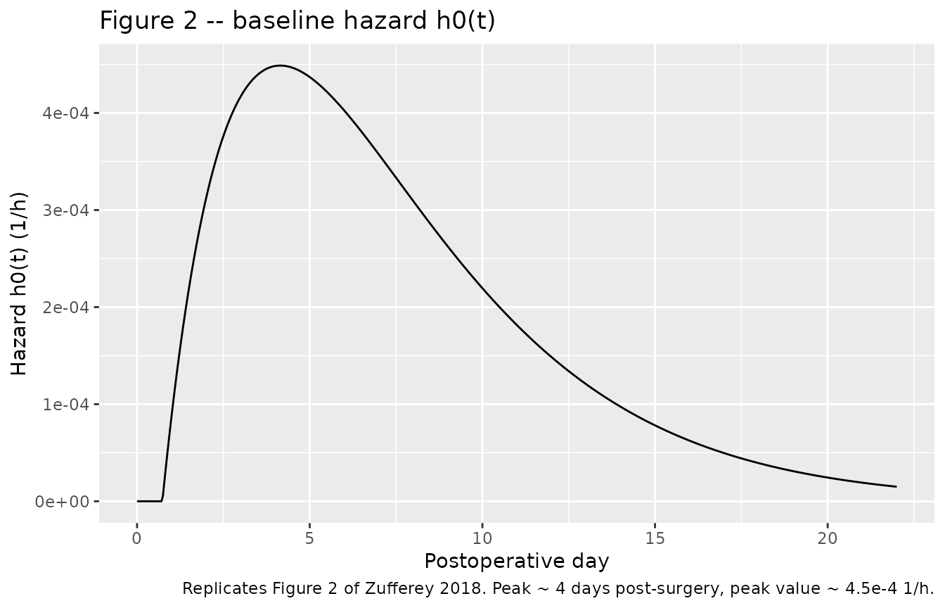
Replicate Figure 1 – Kaplan-Meier of % without major bleeding
Figure 1 shows the percentage of patients without major bleeding versus postoperative day. We construct simulated Kaplan-Meier curves from the typical-value survival trajectory of the virtual pooled cohort.
sim |>
  filter(time %% 24 == 0) |>
  group_by(time) |>
  summarise(S_mean = mean(sur), .groups = "drop") |>
  mutate(time_days = time / 24) |>
  ggplot(aes(time_days, 100 * S_mean)) +
  geom_line() +
  scale_y_continuous(limits = c(85, 100)) +
  labs(x = "Postoperative day", y = "% without major bleeding",
       title = "Figure 1 -- mean simulated survival",
       caption = "Cohort-averaged S(t); replicates Figure 1 of Zufferey 2018 (KM curve, ~95% at day 11).")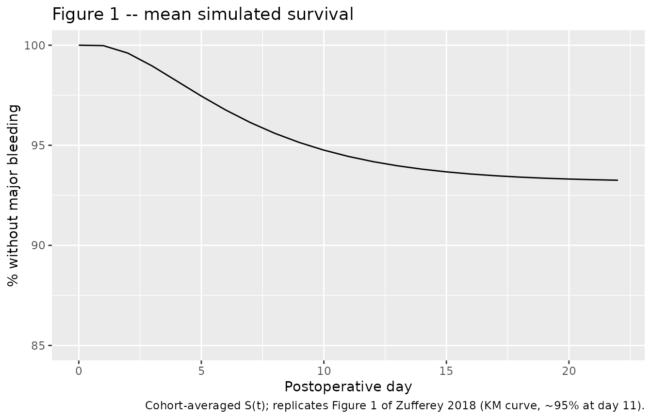
Replicate Figure 3 – LBM, sex, and AUCinf effect panels
Figure 3 of Zufferey 2018 shows, for each combination of sex (rows) and AUCinf level (columns), the probability of avoiding major bleeding for LBM = 30, 40, 50, 60, 70 kg.
auc_levels <- c(5, 8.5, 15)
lbm_levels <- c(30, 40, 50, 60, 70)
sex_levels <- c(0L, 1L)

grid_subjects <- expand.grid(
  AUC = auc_levels,
  LBM = lbm_levels,
  SEXF = sex_levels
) |>
  mutate(id   = row_number(),
         DOSE = 1.0,
         # Force AUCinf = AUC by setting CRCL so that CL = DOSE / AUC = 1 / AUC
         # CL = 0.34 * (CRCL/60)^0.485 => CRCL = 60 * (CL/0.34)^(1/0.485)
         CL_target = 1 / AUC,
         CRCL = 60 * (CL_target / 0.34)^(1 / 0.485))
ev_grid <- crossing(grid_subjects, obs_grid) |>
  select(id, time, evid, amt, DOSE, CRCL, LBM, SEXF, AUC) |>
  as.data.frame()
sim_grid <- rxode2::rxSolve(mod_typ, events = ev_grid,
                            keep = c("DOSE", "CRCL", "LBM", "SEXF", "AUC")) |>
  as.data.frame() |>
  mutate(sex_lab = ifelse(SEXF == 1L, "Female", "Male"),
         auc_lab = paste0("AUC = ", AUC, " mg*h/L"),
         lbm_lab = factor(LBM, levels = lbm_levels))
#> ℹ omega/sigma items treated as zero: 'etalcl'

sim_grid |>
  filter(time %% 24 == 0) |>
  mutate(time_days = time / 24) |>
  ggplot(aes(time_days, 100 * sur, colour = lbm_lab, group = lbm_lab)) +
  geom_line() +
  facet_grid(sex_lab ~ auc_lab) +
  scale_y_continuous(limits = c(70, 100)) +
  scale_colour_brewer(palette = "RdYlBu", direction = -1, name = "LBM (kg)") +
  labs(x = "Postoperative day", y = "% without major bleeding",
       title = "Figure 3 -- effect of LBM, sex, and AUCinf",
       caption = "Replicates Figure 3 of Zufferey 2018.")
#> Warning: Removed 29 rows containing missing values or values outside the scale range
#> (`geom_line()`).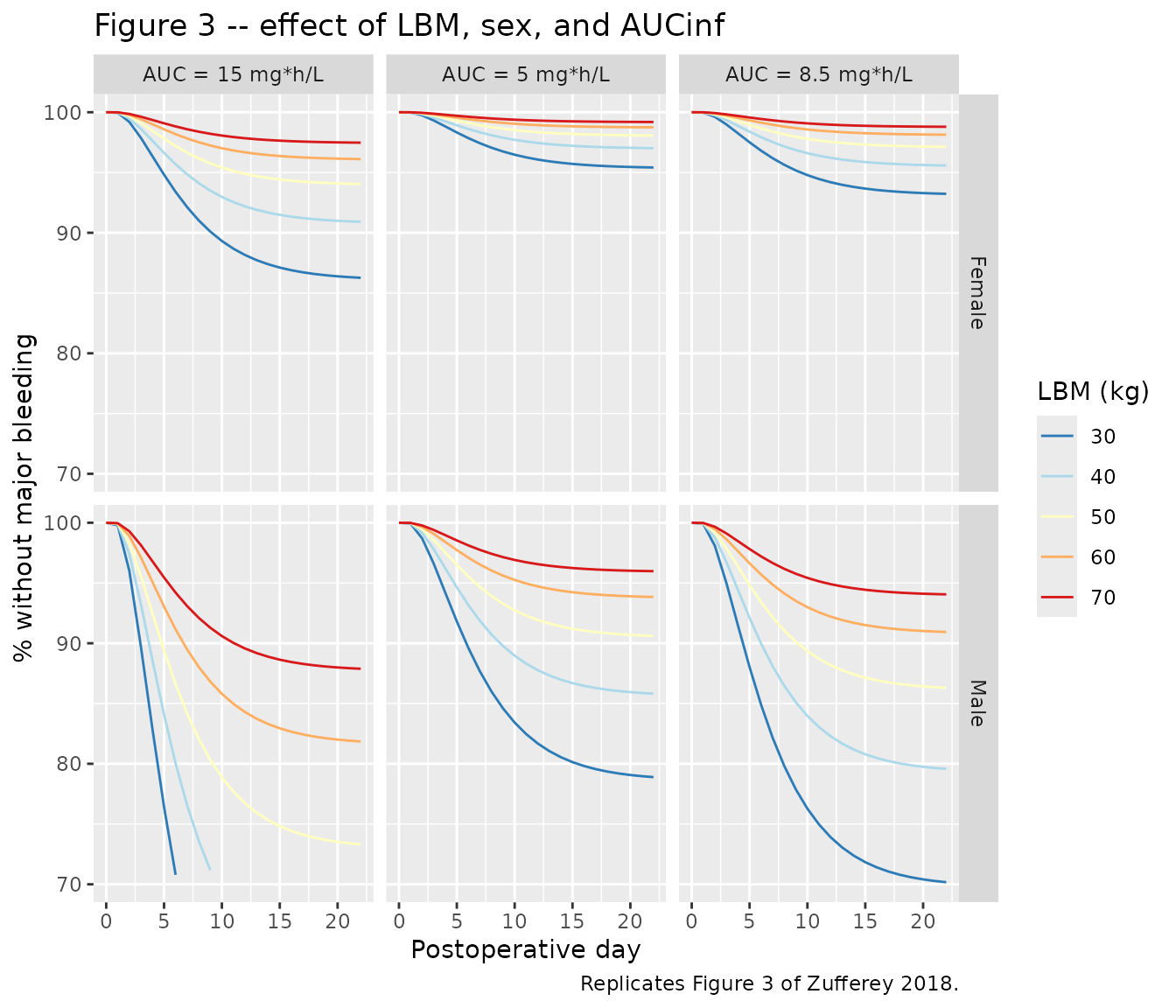
Replicate Table 4 – probability of bleeding at day 11 by dose, sex, and renal function
Table 4 reports the simulated probability of major bleeding at day 11 for the 1.5 mg and 2.5 mg fondaparinux regimens, stratified by sex and renal function (CrCl_Wt; defined with total body weight). The paper draws bootstrap subjects from the actual cohort distribution; we approximate this using the virtual cohort built above, separating by CrCl_LBW <= 30 vs > 30 mL/min as a proxy for the paper’s CrCl_Wt strata (the proxy is approximate because CrCl_Wt and CrCl_LBW differ by the LBW/Wt ratio, which is sex-dependent).
day11_h <- 24 * 11
day11 <- sim |>
  filter(time == day11_h) |>
  mutate(
    sex_lab  = ifelse(SEXF == 1L, "Women", "Men"),
    dose_lab = paste0("Fondaparinux ", DOSE, " mg")
  )

# Overall (matching the unstratified rows of Table 4)
overall <- day11 |>
  group_by(dose_lab) |>
  summarise(p_bleed_pct = 100 * (1 - mean(sur)), .groups = "drop")
knitr::kable(overall, digits = 1,
caption = "Simulated probability (%) of major bleeding at day 11, overall by dose.")| dose_lab | p_bleed_pct |
|---|---|
| Fondaparinux 1.5 mg | 4.7 |
| Fondaparinux 2.5 mg | 6.1 |
# By sex and dose (matches the women / men rows of Table 4)
sex_dose <- day11 |>
  group_by(sex_lab, dose_lab) |>
  summarise(p_bleed_pct = 100 * (1 - mean(sur)), n = n(), .groups = "drop")
knitr::kable(sex_dose, digits = 1,
caption = "Simulated probability (%) of major bleeding at day 11 by sex and dose.")| sex_lab | dose_lab | p_bleed_pct | n |
|---|---|---|---|
| Men | Fondaparinux 1.5 mg | 9.3 | 102 |
| Men | Fondaparinux 2.5 mg | 11.5 | 150 |
| Women | Fondaparinux 1.5 mg | 3.1 | 298 |
| Women | Fondaparinux 2.5 mg | 4.4 | 450 |
The paper’s Table 4 (CrCl_Wt strata) for context:
| Subgroup | CrCl_Wt 20-50 mL/min | CrCl_Wt > 50 mL/min |
|---|---|---|
| Pooled, 2.5 mg | 6.5% (6.2-6.9) | 4.2% (4.0-4.4) |
| Pooled, 1.5 mg | 3.8% (3.7-4.0) | 2.8% (2.7-3.0) |
| Women, 2.5 mg | 5.9% (5.5-6.1) | 3.4% (3.2-3.5) |
| Women, 1.5 mg | 3.5% (3.4-3.7) | 2.3% (2.2-2.4) |
| Men, 2.5 mg | 11.6% (10.3-12.7) | 6.8% (6.4-7.3) |
| Men, 1.5 mg | 7.4% (6.8-8.0) | 5.0% (4.7-5.3) |
Compare AUCinf summary against Table 1
Table 1 reports a pooled-cohort mean AUCinf of 8.5 +/- 3.4 mg*h/L (range 2.7-27). We compute simulated AUCinf at the same per-subject level and compare.
auc_summary <- events |>
  distinct(id, DOSE, CRCL, LBM, SEXF, study) |>
  mutate(cl_typical = 0.34 * (CRCL / 60)^0.485,
         auc_inf    = DOSE / cl_typical) |>
  group_by(study) |>
  summarise(n = n(),
            mean_auc = mean(auc_inf),
            sd_auc   = sd(auc_inf),
            min_auc  = min(auc_inf),
            max_auc  = max(auc_inf),
            .groups  = "drop")
knitr::kable(auc_summary, digits = 2,
caption = "Simulated AUCinf summary by virtual study cohort (typical-value clearance, no IIV).")| study | n | mean_auc | sd_auc | min_auc | max_auc |
|---|---|---|---|---|---|
| POP-A-RIX | 600 | 8.86 | 2.16 | 5.39 | 14.40 |
| PROPICE | 400 | 6.73 | 1.05 | 5.13 | 10.52 |
Reported values for context (Table 1): POP-A-RIX 9.3 +/- 3.4, PROPICE 6.4 +/- 1.9, pooled 8.5 +/- 3.4 mg*h/L.
Assumptions and deviations
-
Drug encoded as the post-surgery TTE model only.
This package extracts the parametric survival model published in the
main text. The pharmacokinetic sub-equation
CL = 0.34 * (CrCl_LBW/60)^0.485 * exp(eta)is embedded so that AUCinf can be derived inside the model from the user-supplied daily dose and CrCl_LBW, exactly as in the paper’s simulation procedure (page 5). The fuller PK structural model that produced this clearance term is described in the paper’s online Supporting Information (Table S1), which was not on disk at extraction time; users who need concentration-time profiles (rather than just AUCinf-driven hazard) should consult the upstream popPK references (Delavenne 2010 and Delavenne 2012, cited as references 7 and 8 of Zufferey 2018). -
Baseline hazard functional form derived from the closed-form
Hz(t). The typeset h0(t) on page 6 reads “h0(t) = theta1 *
theta2 * t * exp(-theta2 * (t - theta3))“, but the published closed-form
cumulative hazard
Hz(theta3) = 0(page 7) implies h0 must equal 0 on[0, theta3]. The only form of h0 that integrates to the published Hz is the gamma-density formh0(t) = theta1 * theta2 * (t - theta3) * exp(-theta2 * (t - theta3))fort > theta3and 0 otherwise. This shape also matches Figure 2 (peak ~ 4 days post-surgery; peak hazard ~ 3.5e-4 1/h ~ theta1 / e). The model file uses this derived form. -
Sex encoding inverted. The source paper uses
SEX = 1for male,SEX = 0for female (Table 3 footnote a). The canonical nlmixr2lib covariate isSEXF(1 = female, 0 = male; seeinst/references/covariate-columns.md). The hazard log-coefficiente_sexf_bleed = +1.62is applied as `e_sexf_bleed- (1 - SEXF)
insidemodel()` so the paper’s published positive value and male-reference interpretation are preserved.
- (1 - SEXF)
- CrCl_LBW vs CrCl_Wt. The model’s CRCL column carries Cockcroft-Gault creatinine clearance computed with lean body weight as the body-size descriptor (the form used in the PK clearance equation). Table 4 of the source paper, by contrast, reports bleeding-probability strata in terms of CrCl_Wt (total body weight); the two scales differ by the LBW/Wt ratio (sex-dependent). The vignette’s stratified bleeding-probability table is therefore an approximation rather than a one-to-one replication of Table 4.
-
PK IIV applied; hazard parameters have no IIV. The
clearance term carries the published CV% = 34 inter-individual
variability as
omega^2 = log(1 + 0.34^2) = 0.10936. The hazard parameters (theta1,theta2,theta3,beta1,beta2,beta3) carry no random effects – Table 3 reports only point estimates and bootstrap 95% CIs, consistent with a typical-value hazard. - Virtual cohort. Sex-conditional LBM and study-conditional CrCl distributions are approximated from the Table 1 summary statistics; the per-subject joint distribution from the actual POP-A-RIX / PROPICE cohorts is not publicly available. Bleeding-probability summaries from the virtual cohort therefore differ from the paper’s bootstrap-based Table 4 values by the discrepancy between the approximated marginals and the true joint distribution.
- NCA validation not applicable. The source paper reports survival / hazard outputs rather than drug-concentration NCA values; PKNCA is omitted. AUCinf is validated against Table 1 summary statistics instead.