Model and source
- Citation: Le J, Huynh J, Vo B, Mai A, Mak RH, Momper JD, Capparelli EV, Harvey H, Avedissian S, Bradley E, Sitapati A, Singh K, Bradley JS. Variability in Meropenem Distribution and Clearance in Children with Sepsis: Population-Based Pharmacokinetics with Assessment of Renal Biomarkers. Clin Pharmacokinet. 2025;64(5):769-777. doi:10.1007/s40262-025-01495-3
- Description: Two-compartment IV population PK model for meropenem in critically ill children with and without sepsis (4 weeks to <21 years) given 20 mg/kg every 8 h as 30-min infusions (Le 2025). Central and peripheral volumes scale linearly with body weight and clearance and intercompartmental clearance allometrically (exponent 0.75), all with reference weight 70 kg. The central volume additionally increases linearly with serum cystatin C (normalised to 0.45 mg/L) and clearance follows a power function of modified-Schwartz eGFR (reference 140 mL/min/1.73 m^2). A single random effect is shared by the central and peripheral volumes; residual error is proportional.
- Article: https://doi.org/10.1007/s40262-025-01495-3 (open access, PMC12064575)
- Supplement (Online Resources 1-5): electronic supplementary material of the article
Le 2025 is a prospective population PK study of IV meropenem in critically ill children with sepsis or septic shock (cases) and matched children receiving meropenem without sepsis (controls). Its novelty is the screening of renal biomarkers, serum creatinine, serum cystatin C and serum neutrophil gelatinase-associated lipocalin (NGAL), as covariates. The final model (Table 2) is a two-compartment model with:
- body-size scaling:
(WT/70)on both volumes and(WT/70)^0.75on CL and Q; - serum cystatin C as a linear effect on the central volume,
V1 = 9.74 * (WT/70) * (1 + 0.449 * CYSC/0.45); - modified-Schwartz eGFR as a power effect on clearance,
CL = 9.72 * (WT/70)^0.75 * (eGFR/140)^0.169.
Population
Twenty-seven children (19 cases, 8 controls) contributed 309 meropenem concentrations (271 from cases) between March 2019 and January 2023 at Rady Children’s Hospital, San Diego (Le 2025 Results, Table 1). Median age was 11.8 years (range 0.6-19.6), median weight 36.3 kg (7.2-98.0), and 67% were male. Seventy-four percent were Hispanic; 70% Caucasian and 30% other or unknown race. Eleven children (all cases) received vasopressors; 88% of controls had appendicitis. All received meropenem 20 mg/kg (maximum 2000 mg) every 8 h as a 30-min infusion. Renal function ranged from acute kidney injury to augmented renal clearance: modified-Schwartz eGFR median 138.9 (22.9-364.8) mL/min/1.73 m^2, serum creatinine 0.33 (0.09-2.57) mg/dL, serum cystatin C 451.1 (178.3-1824.1) ng/mL (Online Resource 3).
The same information is available programmatically via
readModelDb("Le_2025_meropenem")()$population.
Source trace
| Equation / parameter | Value | Source location |
|---|---|---|
lvc (thetaV1) |
log(9.74) L |
Table 2 |
lvp (thetaV2) |
log(4.53) L |
Table 2 |
lcl (thetaCL) |
log(9.72) L/h |
Table 2 |
lq (thetaQ) |
log(1.66) L/h |
Table 2 |
e_wt_cl_q |
fixed(0.75) |
Methods (Pharmacokinetic Modeling); Table 2 footnote |
e_wt_vc_vp |
fixed(1) |
Methods; Table 2 footnote |
e_cysc_vc (thetaV1-SCys) |
0.449 | Table 2 |
e_crcl_cl (thetaCL-eGFR-MS) |
0.169 | Table 2 |
etalcl |
0.487 (variance) | Table 2 row ‘etaCL’ |
etalvc (shared by V1 and V2) |
0.306 (variance) | Table 2 row ‘etaV1, etaV2’; Results ‘assumed to be equal’ |
propSd |
sqrt(0.133) = 0.3647 |
Table 2 row ‘epsilon’ |
| V1 equation | 9.74*(WT/70)*(1+0.449*CYSC/0.45) |
Table 2 footnote |
| V2 equation | 4.53*(WT/70) |
Table 2 footnote |
| CL equation | 9.72*(WT/70)^0.75*(CRCL/140)^0.169 |
Table 2 footnote |
| Q equation | 1.66*(WT/70)^0.75 |
Table 2 footnote |
| eGFR (modified Schwartz) | 0.413 * height (cm) / SCr (mg/dL) |
Online Resource 1 |
| Two-compartment structure, first-order elimination | n/a | Methods; Results |
| Proportional residual error | n/a | Methods (FOCE with ETA-EPS interaction); Figure 1a |
Typical-value checks against the published post hoc parameters
Online Resource 3 tabulates the empirical Bayes (post hoc) estimates
of each PK parameter per kilogram. The intercompartmental clearance has
no random effect, so its per-kilogram value depends on weight alone,
Q/WT = (1.66/70) * (70/WT)^0.25, and the published range
must be reproduced exactly at the cohort’s lightest (7.2 kg) and
heaviest (98.0 kg) child. The peripheral volume per kilogram,
V2/WT = 4.53/70, has no covariate at all, so its typical
value must equal the published median up to the shared random
effect.
mod <- readModelDb("Le_2025_meropenem")
ui <- rxode2::rxode(mod)
#> ℹ parameter labels from comments will be replaced by 'label()'
th <- ui$theta

# Closed-form parameters straight from the Table 2 footnote, written out
# independently of the model object so the comparison below can go red.
le_typical <- function(WT, CYSC, CRCL) {
  data.frame(
    WT = WT, CYSC = CYSC, CRCL = CRCL,
    cl_kg = 9.72 * (WT / 70)^0.75 * (CRCL / 140)^0.169 / WT,
    v1_kg = 9.74 * (WT / 70) * (1 + 0.449 * CYSC / 0.45) / WT,
    v2_kg = 4.53 * (WT / 70) / WT,
    q_kg  = 1.66 * (WT / 70)^0.75 / WT
  )
}

# Same quantities from the packaged model, typical values (etas = 0).
ev_typ <- data.frame(
  id = 1:4, time = 0, evid = 0, amt = 0, cmt = "central",
  WT = c(7.2, 98.0, 36.3, 42.4),
  CYSC = c(0.4511, 0.4511, 0.4511, 0.8010),
  CRCL = c(138.92, 138.92, 138.92, 140.06)
)
typ_mod <- rxode2::rxSolve(rxode2::zeroRe(mod), events = ev_typ,
                           returnType = "data.frame") |>
  dplyr::transmute(id, cl_kg = cl / ev_typ$WT[id], v1_kg = vc / ev_typ$WT[id],
                   v2_kg = vp / ev_typ$WT[id], q_kg = q / ev_typ$WT[id])
#> ℹ parameter labels from comments will be replaced by 'label()'
#> ℹ omega/sigma items treated as zero: 'etalcl', 'etalvc'
#> Warning: multi-subject simulation without without 'omega'
typ_cf <- le_typical(ev_typ$WT, ev_typ$CYSC, ev_typ$CRCL)

# The packaged model reproduces the printed equations (numerical identity).
stopifnot(
  max(abs(typ_mod$cl_kg / typ_cf$cl_kg - 1)) < 1e-8,
  max(abs(typ_mod$v1_kg / typ_cf$v1_kg - 1)) < 1e-8,
  max(abs(typ_mod$v2_kg / typ_cf$v2_kg - 1)) < 1e-8,
  max(abs(typ_mod$q_kg / typ_cf$q_kg - 1)) < 1e-8
)

# Q/kg at the weight extremes reproduces Online Resource 3's range 0.022-0.042
# L/h/kg to the printed precision, and at the median weight its median 0.028.
q_range <- round(typ_mod$q_kg[1:3], 3)
stopifnot(
  isTRUE(all.equal(q_range[2], 0.022)),
  isTRUE(all.equal(q_range[1], 0.042)),
  isTRUE(all.equal(q_range[3], 0.028))
)

typ_cf |>
  dplyr::mutate(
    subject = c("Lightest child (7.2 kg)", "Heaviest child (98 kg)",
                "Median covariates (all)", "Median covariates (controls)"),
    dplyr::across(dplyr::ends_with("_kg"), \(x) signif(x, 3))
  ) |>
  dplyr::select(subject, WT, CYSC, CRCL, cl_kg, v1_kg, v2_kg, q_kg) |>
  dplyr::rename(
    "Subject" = subject, "WT (kg)" = WT, "CYSC (mg/L)" = CYSC,
    "eGFR (mL/min/1.73 m^2)" = CRCL, "CL (L/h/kg)" = cl_kg,
    "V1 (L/kg)" = v1_kg, "V2 (L/kg)" = v2_kg, "Q (L/h/kg)" = q_kg
  ) |>
knitr::kable(caption = "Typical-value parameters per kilogram from the packaged model.")| Subject | WT (kg) | CYSC (mg/L) | eGFR (mL/min/1.73 m^2) | CL (L/h/kg) | V1 (L/kg) | V2 (L/kg) | Q (L/h/kg) |
|---|---|---|---|---|---|---|---|
| Lightest child (7.2 kg) | 7.2 | 0.4511 | 138.92 | 0.245 | 0.202 | 0.0647 | 0.0419 |
| Heaviest child (98 kg) | 98.0 | 0.4511 | 138.92 | 0.127 | 0.202 | 0.0647 | 0.0218 |
| Median covariates (all) | 36.3 | 0.4511 | 138.92 | 0.163 | 0.202 | 0.0647 | 0.0279 |
| Median covariates (controls) | 42.4 | 0.8010 | 140.06 | 0.157 | 0.250 | 0.0647 | 0.0269 |
At the median covariates the typical values are CL 0.163 L/h/kg, V1 0.202 L/kg, V2 0.065 L/kg and Q 0.028 L/h/kg, against published post hoc medians of 0.15, 0.23, 0.06 and 0.028 (Online Resource 3, all participants). The post hoc medians of 27 children carry the random effects, so agreement within the IIV (CV about 80% on CL and 60% on the volumes) is what is expected; the Q identity is exact.
Virtual cohort
Individual data are not public. The virtual cohort below draws weight, serum cystatin C and eGFR independently from log-normal distributions centred on the published medians, with spreads chosen so the 27-child published ranges sit near the 2nd and 98th percentiles, truncated to the observed ranges. Covariates are held constant over the three simulated days (the paper used time-varying values).
set.seed(2025)
rxode2::rxSetSeed(2025)
n_sub <- 200L

rtrunc_lnorm <- function(n, median, lo, hi) {
  sdlog <- log(hi / lo) / 4
  x <- numeric(0)
  while (length(x) < n) {
    y <- stats::rlnorm(2L * n, log(median), sdlog)
    x <- c(x, y[y >= lo & y <= hi])
  }
  x[seq_len(n)]
}

subj <- tibble::tibble(
  id   = seq_len(n_sub),
  WT   = rtrunc_lnorm(n_sub, 36.3, 7.2, 98.0),
  CYSC = rtrunc_lnorm(n_sub, 0.4511, 0.1783, 1.8241),  # ng/mL / 1000
  CRCL = rtrunc_lnorm(n_sub, 138.92, 22.85, 364.82),
  treatment = "20 mg/kg q8h"
)

# 20 mg/kg (max 2000 mg) every 8 h as 30-min infusions for 3 days (9 doses).
dose_times <- seq(0, 64, by = 8)
doses <- subj |>
  tidyr::expand_grid(time = dose_times) |>
  dplyr::mutate(evid = 1L, cmt = "central", amt = pmin(20 * WT, 2000),
                rate = amt / 0.5)
obs_times <- sort(unique(c(seq(0, 8, by = 0.1), seq(24, 32, by = 0.25),
                           seq(48, 56, by = 0.1))))
obs <- subj |>
  tidyr::expand_grid(time = obs_times) |>
  dplyr::mutate(evid = 0L, cmt = "central", amt = 0, rate = 0)
events <- dplyr::bind_rows(doses, obs) |>
  dplyr::arrange(id, time, dplyr::desc(evid)) |>
  as.data.frame()
stopifnot(!anyDuplicated(unique(events[, c("id", "time", "evid")])))
Simulation
sim <- rxode2::rxSolve(mod, events = events, keep = c("treatment", "WT"),
                       returnType = "data.frame")
#> ℹ parameter labels from comments will be replaced by 'label()'
stopifnot(!anyNA(sim$Cc))
Concentration-time profiles on study days 1 and 3
The paper’s Online Resource 5 shows the individual observed concentrations; the sampling design was pre-dose, 0.5, 1, 2, 4 and 8 h after the start of the first studied infusion and again on days 2 and 3. The panels below show the simulated 5th-95th percentile band and median for the first and the seventh (day 3) dose.
sim |>
  dplyr::filter(time <= 8 | (time >= 48 & time <= 56)) |>
  dplyr::mutate(
    day = ifelse(time <= 8, "Day 1 (first dose)", "Day 3 (seventh dose)"),
    tad = ifelse(time <= 8, time, time - 48)
  ) |>
  dplyr::group_by(day, tad) |>
  dplyr::summarise(
    Q05 = quantile(Cc, 0.05), Q50 = median(Cc), Q95 = quantile(Cc, 0.95),
    .groups = "drop"
  ) |>
  ggplot(aes(tad, Q50)) +
  geom_ribbon(aes(ymin = Q05, ymax = Q95), alpha = 0.25) +
  geom_line() +
  facet_wrap(~day) +
  scale_y_log10() +
  labs(x = "Time after start of infusion (h)", y = "Meropenem (mg/L)",
       title = "Simulated meropenem concentrations, 20 mg/kg q8h",
       caption = "Median and 5th-95th percentiles of 200 virtual children; compare Online Resource 5 of Le 2025.")
#> Warning in scale_y_log10(): log-10 transformation introduced infinite values.
#> log-10 transformation introduced infinite values.
#> log-10 transformation introduced infinite values.
#> log-10 transformation introduced infinite values.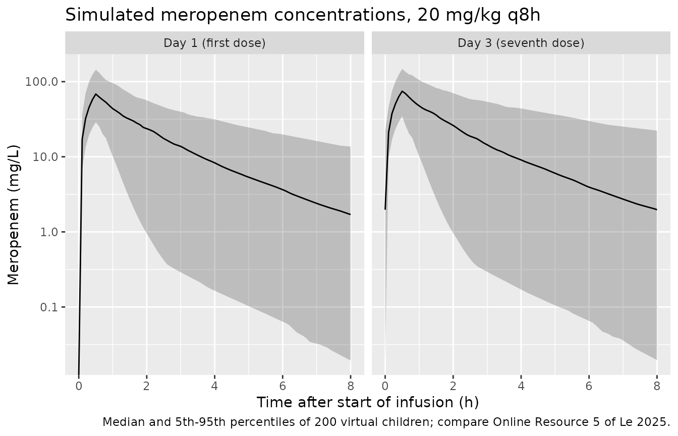
Individual-parameter distribution against Online Resource 3
indiv <- sim |>
  dplyr::distinct(id, WT, cl, vc, vp, q) |>
  dplyr::mutate(cl_kg = cl / WT, v1_kg = vc / WT, v2_kg = vp / WT,
                q_kg = q / WT, ke = cl / vc, thalf = log(2) / ke)

published_or3 <- tibble::tribble(
  ~parameter,          ~pub_median, ~pub_min, ~pub_max,
  "CL (L/h/kg)",        0.15,        0.05,     0.49,
  "V1 (L/kg)",          0.23,        0.07,     0.57,
  "V2 (L/kg)",          0.06,        0.03,     0.14,
  "Q (L/h/kg)",         0.028,       0.022,    0.042,
  "ke (1/h)",           0.66,        0.20,     2.33,
  "t1/2 = 0.693/ke (h)", 1.05,       0.30,     3.48
)
sim_or3 <- tibble::tibble(
  parameter = published_or3$parameter,
  sim_median = c(median(indiv$cl_kg), median(indiv$v1_kg), median(indiv$v2_kg),
                 median(indiv$q_kg), median(indiv$ke), median(indiv$thalf)),
  sim_p05 = c(quantile(indiv$cl_kg, 0.05), quantile(indiv$v1_kg, 0.05),
              quantile(indiv$v2_kg, 0.05), quantile(indiv$q_kg, 0.05),
              quantile(indiv$ke, 0.05), quantile(indiv$thalf, 0.05)),
  sim_p95 = c(quantile(indiv$cl_kg, 0.95), quantile(indiv$v1_kg, 0.95),
              quantile(indiv$v2_kg, 0.95), quantile(indiv$q_kg, 0.95),
              quantile(indiv$ke, 0.95), quantile(indiv$thalf, 0.95))
)
or3 <- dplyr::left_join(published_or3, sim_or3, by = "parameter") |>
  dplyr::mutate(ratio = sim_median / pub_median)

# Centre check: a mis-transcribed theta or covariate normaliser (for example
# reading the cystatin C normaliser in ng/mL) moves these medians several-fold.
# The published medians are post hoc estimates from only 27 children (log-scale
# sampling SE of a median about 0.17 for a log-SD of 0.7), and the ratios
# realised here were 0.92-1.16, so the bound is a factor of 1.6.
stopifnot(all(abs(log(or3$ratio)) < log(1.6)))

or3 |>
  dplyr::mutate(dplyr::across(c(sim_median, sim_p05, sim_p95, ratio), \(x) signif(x, 3))) |>
  dplyr::rename(
    "Parameter" = parameter, "Published median" = pub_median,
    "Published min" = pub_min, "Published max" = pub_max,
    "Simulated median" = sim_median, "Simulated P5" = sim_p05,
    "Simulated P95" = sim_p95, "Simulated / published median" = ratio
  ) |>
knitr::kable(caption = "Individual PK parameters: Online Resource 3 post hoc estimates (27 children) vs the 200-child virtual cohort.")| Parameter | Published median | Published min | Published max | Simulated median | Simulated P5 | Simulated P95 | Simulated / published median |
|---|---|---|---|---|---|---|---|
| CL (L/h/kg) | 0.150 | 0.050 | 0.490 | 0.1380 | 0.0487 | 0.6390 | 0.919 |
| V1 (L/kg) | 0.230 | 0.070 | 0.570 | 0.2220 | 0.0939 | 0.5750 | 0.963 |
| V2 (L/kg) | 0.060 | 0.030 | 0.140 | 0.0698 | 0.0296 | 0.1690 | 1.160 |
| Q (L/h/kg) | 0.028 | 0.022 | 0.042 | 0.0284 | 0.0228 | 0.0369 | 1.010 |
| ke (1/h) | 0.660 | 0.200 | 2.330 | 0.6080 | 0.1850 | 2.8600 | 0.921 |
| t1/2 = 0.693/ke (h) | 1.050 | 0.300 | 3.480 | 1.1400 | 0.2420 | 3.7500 | 1.090 |
PKNCA validation
The paper does not report non-compartmental parameters, so there is
no published NCA table to compare against. PKNCA is used instead to
check the steady-state mass balance over the day-3 dosing interval
(48-56 h): at steady state, AUC_tau = dose / CL for every
child, an identity that uses each subject’s own simulated clearance.
sim_nca <- sim |>
  dplyr::filter(!is.na(Cc), time >= 48, time <= 56) |>
  dplyr::mutate(Cc = pmax(Cc, 0)) |>
  dplyr::select(id, time, Cc, treatment)

dose_nca <- doses |>
  dplyr::filter(time == 48) |>
  dplyr::select(id, time, amt, treatment) |>
  as.data.frame()

conc_obj <- PKNCA::PKNCAconc(sim_nca, Cc ~ time | treatment + id)
dose_obj <- PKNCA::PKNCAdose(dose_nca, amt ~ time | treatment + id)
intervals <- data.frame(start = 48, end = 56, cmax = TRUE, tmax = TRUE,
                        cmin = TRUE, auclast = TRUE)
nca_res <- PKNCA::pk.nca(PKNCA::PKNCAdata(conc_obj, dose_obj, intervals = intervals,
                                          options = list(auc.method = "lin up/log down")))

nca_wide <- as.data.frame(nca_res) |>
  dplyr::select(id, PPTESTCD, PPORRES) |>
  tidyr::pivot_wider(names_from = PPTESTCD, values_from = PPORRES) |>
  dplyr::left_join(dose_nca |> dplyr::select(id, amt), by = "id") |>
  dplyr::left_join(indiv |> dplyr::select(id, cl), by = "id") |>
  dplyr::mutate(auc_ratio = auclast / (amt / cl))

# Same drawn parameters on both sides: the residual is trapezoid error on the
# 0.1-h grid plus any approach to steady state still incomplete after six
# doses in the slowest-clearing children.
stopifnot(
  abs(median(nca_wide$auc_ratio) - 1) < 0.02,
  quantile(abs(nca_wide$auc_ratio - 1), 0.9) < 0.05
)

nca_wide |>
  dplyr::summarise(
    dplyr::across(c(cmax, cmin, auclast, auc_ratio),
                  list(median = median, p05 = \(x) quantile(x, 0.05),
                       p95 = \(x) quantile(x, 0.95)))
  ) |>
  tidyr::pivot_longer(dplyr::everything(),
                      names_to = c("parameter", "stat"),
                      names_pattern = "^(.*)_(median|p05|p95)$") |>
  tidyr::pivot_wider(names_from = stat, values_from = value) |>
  dplyr::mutate(
    parameter = dplyr::recode(parameter,
      cmax = "Cmax (mg/L)", cmin = "Cmin (mg/L)",
      auclast = "AUC0-8,ss (mg*h/L)", auc_ratio = "AUC0-8,ss / (dose/CL)"),
    dplyr::across(c(median, p05, p95), \(x) signif(x, 3))
  ) |>
  dplyr::rename("NCA parameter" = parameter, "Median" = median,
                "P5" = p05, "P95" = p95) |>
knitr::kable(caption = "PKNCA over the day-3 dosing interval (48-56 h), 20 mg/kg q8h.")| NCA parameter | Median | P5 | P95 |
|---|---|---|---|
| Cmax (mg/L) | 74.60 | 34.6000 | 148.0 |
| Cmin (mg/L) | 1.97 | 0.0196 | 22.2 |
| AUC0-8,ss (mg*h/L) | 145.00 | 31.2000 | 408.0 |
| AUC0-8,ss / (dose/CL) | 1.00 | 0.9950 | 1.0 |
Assumptions and deviations
-
Cystatin C units. Table 2 states that SCys is in
ng/mL, but the V1 equation divides SCys by 0.45. Read literally in ng/mL
the ratio would be about 1000 at the cohort median (451 ng/mL) and V1
would be several hundred times too large. The normaliser 0.45 equals the
cohort median expressed in mg/L (0.451 mg/L), so the model uses the
canonical
CYSCcolumn in mg/L (CYSC = SCys [ng/mL] / 1000). The typical V1 per kilogram at the median covariates (0.20 L/kg) then agrees with the published post hoc median of 0.23 L/kg. Note that the study’s research ELISA reads lower than the clinical immunoturbidimetric assays behind the adult reference range of about 0.6-1.1 mg/L, so cystatin C values from a clinical assay should not be plugged in without considering the assay difference. -
Variance scale of the random effects. Table 2 does
not say whether the eta and epsilon rows are variances or standard
deviations. They are taken as the raw NONMEM variances. The bootstrap
95% CI relative width of the ‘etaV1, etaV2’ row, (0.464 - 0.153)/0.287 =
1.08, matches the width expected for a variance estimated from 27
subjects, 3.92 * sqrt(2/27) = 1.07, and is twice the width expected for
a standard deviation (0.53). The etaCL row (0.83) also sits nearer the
variance prediction. The residual row is read on the same scale
(proportional SD
sqrt(0.133) = 36.5%). - Shared random effect on V1 and V2. Results state that the inter-subject variability of V1 and V2 “was assumed to be equal”, and Table 2 reports a single row ‘etaV1, etaV2’. The model uses one eta for both volumes rather than two independent etas with equal variance; Online Resource 3 reports identical quartile-wise case-versus-control p-values for V1 and V2 (0.011, <0.001, 0.73, 0.057), which a shared eta produces and two independent etas would not.
- Proportional residual error. The paper says proportional and additive error models were explored but not which was retained. A single epsilon is reported, estimation used FOCE with ETA-EPS interaction (which matters only for a prediction-dependent error), and the Figure 1a observed-versus-IPRED scatter widens with concentration, so a proportional error is used.
- Cases versus controls. The final model has no sepsis covariate. Online Resource 3 shows lower post hoc CL in cases than controls (0.14 vs 0.29 L/h/kg) with near-identical median eGFR (138.9 vs 140.1), so that difference sits in the random effects and the model’s covariates do not reproduce it. Part of the V1 difference (0.19 vs 0.29 L/kg) is carried by cystatin C: the typical V1 at the control median cystatin C (0.80 mg/L) and weight is 0.25 L/kg against 0.20 L/kg at the case median (0.43 mg/L).
-
eGFR equation for young adults. The two
participants aged 18 years or older had eGFR computed by CKD-EPI rather
than the modified Schwartz equation (Online Resource 1); the model uses
whatever value is supplied in
CRCL. - Virtual cohort. Weight, cystatin C and eGFR are drawn independently (the paper reports no correlations), truncated to the published ranges, and held constant in time; the paper used time-varying biomarker values with nearest-value carry-forward/backward.
- No erratum or correction notice for the article was found (checked 2026-11-04).