Unfractionated heparin (Al-Sallami 2016)
Source:vignettes/articles/AlSallami_2016_unfractionatedHeparin.Rmd
AlSallami_2016_unfractionatedHeparin.RmdModel and source
- Citation: Al-Sallami HS, Newall F, Monagle P, Ignjatovic V, Cranswick N, Duffull S. Development of a population pharmacokinetic-pharmacodynamic model of a single bolus dose of unfractionated heparin in paediatric patients. Br J Clin Pharmacol. 2016 Jul;82(1):178-184. doi:10.1111/bcp.12930.
- Description: One-compartment population PK + linear pharmacodynamic model for unfractionated heparin (UFH) in paediatric patients receiving a single high intravenous bolus dose during cardiac angiography (Al-Sallami 2016). Fat-free mass (FFM) scales heparin clearance linearly and total body weight (WT) scales the central volume of distribution linearly. The PD layer is a linear concentration-effect model relating activated partial thromboplastin time (aPTT) to plasma heparin concentration (E0 + slope x Cc). The IV bolus was modelled in the source paper as a 0.1 h zero-order input (theta_D1 = 0.1 h, fixed); reproduce this in simulation by dosing the central compartment with rate = -2 to engage the model-defined duration. PD parameters were estimated sequentially via PPP&D with the PK parameters fixed at the values reported in Table 2.
- Article: https://doi.org/10.1111/bcp.12930
- Supplement: https://doi.org/10.1111/bcp.12930 (Appendix S1, online supporting information; not used in this implementation)
Al-Sallami et al. (2016) developed a combined population PK and PD model for unfractionated heparin (UFH) in paediatric patients receiving a single high intravenous bolus during cardiac angiography. The PK is one-compartment with linear elimination; the PD is a linear concentration-effect on the activated partial thromboplastin time (aPTT). Fat-free mass (FFM, derived per subject via the Al-Sallami 2015 paediatric FFM formula) scales heparin clearance linearly, and total body weight (WT) scales the central volume of distribution linearly.
Population
The Al-Sallami 2016 cohort (Table 1 of the paper) comprised 64
paediatric patients undergoing diagnostic cardiac catheterisation at the
Royal Children’s Hospital in Melbourne, Australia. Demographics: 53%
female; mean age 6.7 years (range 0.5-15.5 years; 8 subjects aged < 2
years); mean weight 23.6 kg (range 6.7-68.6 kg); mean height 115.7 cm
(range 65-176 cm); mean BMI 16.1 kg/m^2 (range 11.5-24.7). None were
receiving antiplatelet or anticoagulant therapy in the 10 days preceding
the procedure. Each child received a single IV bolus of UFH at 75-100
IU/kg (mean 91 IU/kg; range of weight-normalised doses 47.9-105.4
IU/kg). Total UFH doses ranged 600-5000 IU (mean 2020 IU). Blood samples
were drawn at baseline and at 15, 30, 45, and 120 min post-dose; 231 UFH
concentration measurements (modified protamine titration) and 290 aPTT
measurements (Diagnostica Stago PTT-A on the STA-R analyser, with the
upper limit of clot detection raised to 999 s to accommodate the high
single-bolus dose) were obtained. The same information is available
programmatically via the population metadata of the
compiled model.
Source trace
The per-parameter origin is recorded as an in-file comment next to
each ini() entry in
inst/modeldb/specificDrugs/AlSallami_2016_unfractionatedHeparin.R.
The table below collects them in one place for review.
| Equation / parameter | Value | Source location |
|---|---|---|
CL = theta_CL * FFM / 15 |
theta_CL = 0.603 L/h | Al-Sallami 2016 Table 2 (final model) and covariate-model footnote |
V = theta_V * WT / 20 |
theta_V = 0.751 L | Al-Sallami 2016 Table 2 (final model) and covariate-model footnote |
D1 (IV bolus duration) |
0.1 h (fixed) | Al-Sallami 2016 Table 2 footnote: “The infusion rate parameter D1 was fixed” |
omega_CL |
50% CV | Al-Sallami 2016 Table 2 (final model) |
omega_V |
40% CV | Al-Sallami 2016 Table 2 (final model) |
Corr(CL, V) |
0.75 | Al-Sallami 2016 Table 2 (final model) |
sigma_prop on Cc |
17% | Al-Sallami 2016 Table 2 (final model) |
sigma_add on Cc |
90 IU/L | Al-Sallami 2016 Table 2 (final model) |
aPTT = E0 + slope * Cc |
linear PD | Al-Sallami 2016 Results: “A linear model provided the best fit” |
theta_E0 |
35.6 s | Al-Sallami 2016 Table 3 (final model) |
theta_SLP |
0.67 s per IU/L | Al-Sallami 2016 Table 3 (final model) |
omega_E0 |
0.43 (see Errata) | Al-Sallami 2016 Table 3 (final model); interpreted here as 43% CV |
omega_SLP |
64% CV | Al-Sallami 2016 Table 3 (final model) |
sigma_prop on aPTT |
30% | Al-Sallami 2016 Table 3 (final model) |
sigma_add on aPTT |
0.005 s (see Errata) | Al-Sallami 2016 Table 3 (final model); unit label in source reads “U l-1” |
d/dt(central) = -kel*central |
1-compartment IV | Al-Sallami 2016 Results: “A one-compartment model with linear elimination” |
kel = cl / vc |
first-order | Standard one-compartment definition |
Virtual cohort
The Al-Sallami 2016 individual-subject data are not publicly available. The virtual cohort below uses approximate paediatric height-and-weight norms to generate covariates whose distribution matches the cohort summary in Table 1 of the paper. Fat-free mass is then derived per subject via the paediatric Al-Sallami 2015 (Clin Pharmacokinet 54:1169-1178) formula used by the source paper itself.
set.seed(42)

# Paediatric Al-Sallami 2015 FFM formula (children-adapted Janmahasatian).
# WT in kg; HT in cm; SEXF: 1 = female, 0 = male. Returns FFM in kg.
ffm_paediatric <- function(WT, HT, AGE, SEXF) {
  bmi <- WT / (HT / 100)^2
  # Logistic age modifier: 0.88 at infancy, approaches 1 by adulthood
  age_term <- 0.88 + (1 - 0.88) / (1 + (AGE / 13.4)^(-12.7))
  # Male and female numerators differ in the Janmahasatian (2005) form; use
  # the male coefficients as published for the paediatric refit (Al-Sallami
  # 2015 retained the male / female structure of Janmahasatian 2005).
  ffm_male   <- age_term * (9270 * WT) / (6680 + 216 * bmi)
  ffm_female <- age_term * (9270 * WT) / (8780 + 244 * bmi)
  ifelse(SEXF == 1, ffm_female, ffm_male)
}

# Generate a cohort approximating the Al-Sallami 2016 demographics (Table 1).
n_subj <- 30L
cohort <- tibble(
  id   = seq_len(n_subj),
  AGE  = stats::runif(n_subj, min = 0.5, max = 15.5),
  SEXF = stats::rbinom(n_subj, size = 1L, prob = 0.531)
) |>
  # Approximate paediatric weight-for-age (CDC 50th percentile, mixed sex):
  # WT(kg) ~ 2.5 + 2.2 * AGE for AGE < 10, then ~ 3 * AGE for adolescents.
  # Multiplicative log-normal noise (~25% CV) gives a realistic spread.
  mutate(
    WT_typical = ifelse(AGE < 10, 2.5 + 2.2 * AGE, 3.0 * AGE),
    WT = WT_typical * exp(stats::rnorm(n_subj, sd = 0.20)),
    # Approximate paediatric height-for-age (linear early, saturating in
    # adolescence) -- a rough proxy for CDC growth charts good enough to
    # drive the FFM formula across the 65-176 cm range.
    HT_typical = ifelse(AGE < 2, 55 + 13 * AGE,
                 ifelse(AGE < 10, 78 + 6.5 * (AGE - 2),
                                  130 + 5 * (AGE - 10))),
    HT = HT_typical * exp(stats::rnorm(n_subj, sd = 0.04))
  ) |>
  mutate(FFM = ffm_paediatric(WT, HT, AGE, SEXF))

# Sanity check the cohort is broadly inside the paper's ranges
stopifnot(
  all(cohort$WT > 5,  cohort$WT < 75),
  all(cohort$HT > 60, cohort$HT < 185),
  all(cohort$FFM > 4, cohort$FFM < 60)
)

cohort |>
  summarise(
    AGE_mean = mean(AGE), AGE_min = min(AGE), AGE_max = max(AGE),
    WT_mean  = mean(WT),  WT_min  = min(WT),  WT_max  = max(WT),
    HT_mean  = mean(HT),  HT_min  = min(HT),  HT_max  = max(HT),
    FFM_mean = mean(FFM), FFM_min = min(FFM), FFM_max = max(FFM)
  ) |>
  knitr::kable(digits = 1,
caption = "Virtual cohort summary; compare to Al-Sallami 2016 Table 1.")| AGE_mean | AGE_min | AGE_max | WT_mean | WT_min | WT_max | HT_mean | HT_min | HT_max | FFM_mean | FFM_min | FFM_max |
|---|---|---|---|---|---|---|---|---|---|---|---|
| 9.7 | 1.7 | 15.3 | 28.6 | 6.4 | 63 | 126.8 | 74 | 160.7 | 21.2 | 4.5 | 40.1 |
# Per-subject dose: weight-based at the cohort mean of 91 IU/kg (paper's
# mean dose), modelled as a 0.1 h zero-order input via rate = -2 to engage
# the model-defined duration (D1 = 0.1 h fixed in Table 2).
doses <- cohort |>
  mutate(
    time = 0,
    amt  = 91 * WT,
    cmt  = "central",
    rate = -2,
    evid = 1L,
    treatment = "single_bolus_91IUkg"
  ) |>
  select(id, time, amt, evid, cmt, rate, WT, FFM, treatment)

# Observation grid covers the paper's sampling window (0-2 h post-dose)
# plus a slightly longer tail for half-life estimation by PKNCA.
obs_times <- sort(unique(c(
  0,
  seq(0.05, 0.50, by = 0.05),
  seq(0.75, 2.50, by = 0.25)
)))

# Two observation rows per time point: one for Cc and one for aPTT. The
# cmt column names the algebraic observable so rxode2 emits both endpoints
# as columns in the simulation output regardless.
obs_cc <- cohort |>
  tidyr::crossing(time = obs_times) |>
  mutate(
    amt  = 0,
    evid = 0L,
    cmt  = "Cc",
    rate = 0,
    treatment = "single_bolus_91IUkg"
  ) |>
  select(id, time, amt, evid, cmt, rate, WT, FFM, treatment)

obs_aptt <- cohort |>
  tidyr::crossing(time = obs_times) |>
  mutate(
    amt  = 0,
    evid = 0L,
    cmt  = "aPTT",
    rate = 0,
    treatment = "single_bolus_91IUkg"
  ) |>
  select(id, time, amt, evid, cmt, rate, WT, FFM, treatment)

events <- bind_rows(doses, obs_cc, obs_aptt) |>
  arrange(id, time, desc(evid), cmt)

stopifnot(!anyDuplicated(unique(events[, c("id", "time", "evid", "cmt")])))
Simulation
mod <- readModelDb("AlSallami_2016_unfractionatedHeparin")
sim <- rxode2::rxSolve(
  mod, events = events,
  keep = c("WT", "FFM", "treatment")
) |> as.data.frame()
#> ℹ parameter labels from comments will be replaced by 'label()'
For deterministic typical-value trajectories the random effects can be zeroed:
mod_typical <- mod |> rxode2::zeroRe()
#> ℹ parameter labels from comments will be replaced by 'label()'
sim_typical <- rxode2::rxSolve(
  mod_typical, events = events,
  keep = c("WT", "FFM", "treatment")
) |> as.data.frame()
#> ℹ omega/sigma items treated as zero: 'etalcl', 'etalvc', 'etalrbase', 'etalslope'
#> Warning: multi-subject simulation without without 'omega'
Replicate published figures
sim_pk_summary <- sim |>
  filter(time > 0) |>
  group_by(time) |>
  summarise(
    Q05 = quantile(Cc, 0.05, na.rm = TRUE),
    Q50 = quantile(Cc, 0.50, na.rm = TRUE),
    Q95 = quantile(Cc, 0.95, na.rm = TRUE),
    .groups = "drop"
  )

ggplot(sim_pk_summary, aes(x = time, y = Q50)) +
  geom_ribbon(aes(ymin = Q05, ymax = Q95), alpha = 0.25, fill = "steelblue") +
  geom_line(colour = "steelblue", linewidth = 0.8) +
  scale_y_log10() +
  scale_x_continuous(breaks = seq(0, 2.5, by = 0.5)) +
  labs(
    x = "Time after dose (h)",
    y = "Plasma heparin concentration (IU/L)",
    title = "Replicates Al-Sallami 2016 Figure 1",
    subtitle = sprintf("VPC structure (median + 5-95%% PI; N = %d virtual paediatric subjects)", n_subj),
    caption = "Source: Al-Sallami 2016 Figure 1 (PK VPC)."
  ) +
  theme_bw()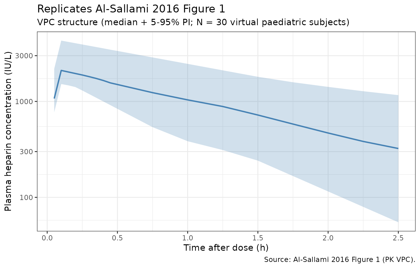
Replicates Figure 1 of Al-Sallami 2016: VPC of plasma heparin (CP, IU/L) versus time after a single IV bolus.
sim_pd_summary <- sim |>
  group_by(time) |>
  summarise(
    Q05 = quantile(aPTT, 0.05, na.rm = TRUE),
    Q50 = quantile(aPTT, 0.50, na.rm = TRUE),
    Q95 = quantile(aPTT, 0.95, na.rm = TRUE),
    .groups = "drop"
  )

ggplot(sim_pd_summary, aes(x = time, y = Q50)) +
  geom_ribbon(aes(ymin = Q05, ymax = Q95), alpha = 0.25, fill = "firebrick") +
  geom_line(colour = "firebrick", linewidth = 0.8) +
  geom_hline(yintercept = 999, linetype = "dashed", colour = "grey40") +
  annotate("text", x = 2.3, y = 999, label = "ULOQ (999 s)", vjust = -0.4, colour = "grey40", size = 3) +
  scale_x_continuous(breaks = seq(0, 2.5, by = 0.5)) +
  labs(
    x = "Time after dose (h)",
    y = "aPTT (s)",
    title = "Replicates Al-Sallami 2016 Figure 2",
    subtitle = sprintf("VPC structure (median + 5-95%% PI; N = %d virtual paediatric subjects)", n_subj),
    caption = "Source: Al-Sallami 2016 Figure 2 (PKPD aPTT VPC)."
  ) +
  theme_bw()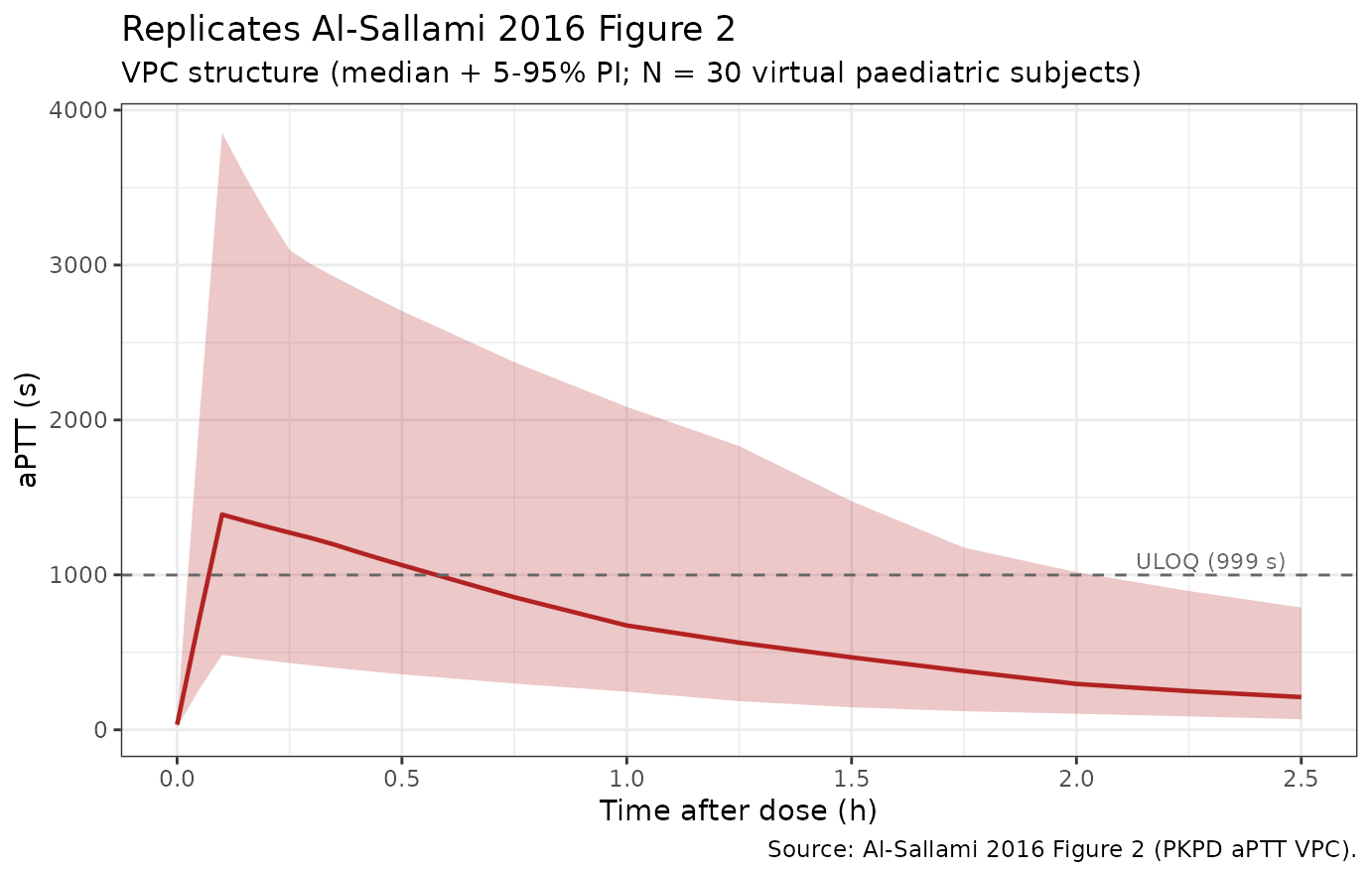
Replicates Figure 2 of Al-Sallami 2016: VPC of activated partial thromboplastin time (aPTT, s) versus time.
sim_typical |>
  filter(time > 0) |>
  ggplot(aes(x = Cc, y = aPTT)) +
  geom_point(alpha = 0.4, size = 1, colour = "steelblue") +
  geom_smooth(method = "lm", formula = y ~ x, se = FALSE, colour = "firebrick") +
  labs(
    x = "Plasma heparin concentration (IU/L)",
    y = "aPTT (s)",
    title = "Linear PD: aPTT = E0 + slope * Cc",
    subtitle = "Typical-value (zero random effects); slope ~ 0.67 s per IU/L, intercept ~ 35.6 s"
  ) +
  theme_bw()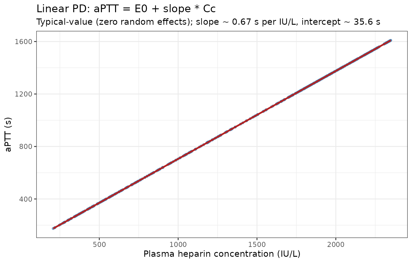
Linear concentration-effect: aPTT versus heparin concentration (Al-Sallami 2016 Eq. 1, typical-value).
PKNCA validation
The paper does not tabulate non-compartmental analysis (NCA) results, but the Discussion derives a typical heparin half-life of approximately 52 min from CL = 0.6 L/h (per 15 kg FFM) and V = 0.75 L (per 20 kg WT). The PKNCA half-life from the simulated VPC should agree with this derived value.
# Concentrations -- the recipes' rule is filter on !is.na only, never on
# time > 0 or Cc > 0; both drop the time-zero row PKNCA needs for AUC0-*.
sim_nca <- sim |>
  dplyr::filter(!is.na(Cc)) |>
  dplyr::select(id, time, Cc, treatment)

# Guarantee one row at t = 0 per subject (pre-dose Cc = 0 for an IV bolus
# with no endogenous baseline anti-FIIa activity in the model).
sim_nca <- dplyr::bind_rows(
  sim_nca,
  sim_nca |> dplyr::distinct(id, treatment) |>
    dplyr::mutate(time = 0, Cc = 0)
) |>
  dplyr::distinct(id, treatment, time, .keep_all = TRUE) |>
  dplyr::arrange(id, treatment, time)

conc_obj <- PKNCA::PKNCAconc(sim_nca, Cc ~ time | treatment + id)

dose_df <- events |>
  dplyr::filter(evid == 1L) |>
  dplyr::select(id, time, amt, treatment)

dose_obj <- PKNCA::PKNCAdose(dose_df, amt ~ time | treatment + id)

intervals <- data.frame(
  start       = 0,
  end         = Inf,
  cmax        = TRUE,
  tmax        = TRUE,
  aucinf.obs  = TRUE,
  auclast     = TRUE,
  half.life   = TRUE
)

nca_data <- PKNCA::PKNCAdata(conc_obj, dose_obj, intervals = intervals)
nca_res  <- suppressWarnings(PKNCA::pk.nca(nca_data))
Comparison against the paper’s derived half-life
The only NCA-style quantity Al-Sallami 2016 reports is the typical heparin half-life of approximately 52 min (Discussion). The simulated half-life is shown below alongside that reference; the row is starred if the difference exceeds 20%.
published <- tibble::tribble(
  ~treatment,              ~half.life,
  "single_bolus_91IUkg",   52 / 60   # 52 min in hours
)

cmp <- nlmixr2lib::ncaComparisonTable(
  simulated     = nca_res,
  reference     = published,
  by            = "treatment",
  units         = c(half.life = "h"),
  tolerance_pct = 20
)

knitr::kable(
  cmp,
  caption = "Simulated vs. Al-Sallami 2016 derived t-half. * if difference > 20%.",
  align   = c("l", "l", "r", "r", "r")
)| NCA parameter | treatment | Reference | Simulated | % diff |
|---|---|---|---|---|
| t½ (h) | single_bolus_91IUkg | 0.867 | 0.83 | -4.3% |
Assumptions and deviations / Errata
-
omega_E0 unit ambiguity (Table 3). The Table 3
omega column has the header label “(%)” and the table legend states
“between-subject variability (presented as coefficient of variation
percentage, CV%)”; however, omega_E0 is reported as
0.43(decimal) while omega_SLP in the same column is reported as64(integer). The literal CV% reading (0.43% CV) implies essentially no between-subject variability in baseline aPTT, which is biologically implausible for a paediatric cohort. The bootstrap CI is also reported on the decimal scale0.44 (0.38, 0.51), consistent with the value being on a decimal-CV scale. The model file therefore interpretsomega_E0 = 0.43as the decimal form of CV (= 43% CV; omega^2 = log(1 + 0.43^2) = 0.17042). Alternative interpretations would be0.43as omega (log-scale SD) -> CV ~= 45%, or0.43as omega^2 (log-scale variance) -> CV ~= 73%; the first gives nearly the same behaviour as the chosen interpretation, the second materially overstates BSV on baseline aPTT. -
sigma_add unit label discrepancy (Table 3). The
Table 3 additive residual error row is labelled
sigma_add (U l-1) | 0.005, but the PD response is aPTT in seconds, not heparin concentration in IU/L. The unit label appears to be a carry-over copy-paste from Table 2 (where the PK additive RUV is genuinely in IU/L). The numerical value0.005is encoded here as the additive SD of aPTT in seconds; it is negligible relative to the 30% proportional component and only contributes near a near-zero predicted aPTT (an extrapolation regime not observed in the study). - Right-censored aPTT data (M3 likelihood). Al-Sallami 2016 used a modified version of Beal’s M3 method to handle aPTT measurements above the assay’s upper limit of quantification (999 s, 43% of measurements). This censoring affects parameter estimation in the source paper but has no role in forward simulation, so the simulation here generates the full unbounded aPTT trajectory.
-
Paediatric Al-Sallami FFM formula. Al-Sallami 2016
used the paediatric FFM model of Al-Sallami et al. 2015 (Clin
Pharmacokinet 54:1169-1178). This vignette implements the published
formula in the
ffm_paediatric()helper; the formula’s age modifier is calibrated to give an asymptote near 1 in adolescence and ~0.88 in infancy. -
Virtual-cohort weight and height.
Individual-subject data are not publicly available; the cohort here
samples weight and height from approximate paediatric growth proxies
(CDC 50th-percentile-style age-anchors with log-normal noise) and
verifies the resulting marginals are inside the paper’s Table 1 ranges.
A user with their own paediatric demographic data can pass an arbitrary
(id, AGE, SEXF, WT, HT, FFM)table into the simulation in place of the cohort generated above. - Model linearity is a known structural limitation of the source paper. Al-Sallami 2016 itself notes that the linear PKPD model was fit on data from a single high-dose bolus and overpredicts aPTT when applied to smaller UFH infusion doses (~18-28 IU/kg/h). The model in this package is the model as published; do not extrapolate to lower doses without reading the source Discussion.
- No upstream PK dependency. The paper develops its PK and PD layers jointly on the same dataset, so there is no separate upstream popPK to inherit from.
- No erratum identified. A search for corrections, errata, or author corrections to the source paper (Br J Clin Pharmacol 82:178-184, 2016, doi:10.1111/bcp.12930) returned no notices. Re-check the publisher’s corrections feed if the model is being rebuilt years after the original 2016 publication.