S-ketamine and S-norketamine (Flint 2017)
Source:vignettes/articles/Flint_2017_s_ketamine.Rmd
Flint_2017_s_ketamine.RmdModel and source
#> ℹ parameter labels from comments will be replaced by 'label()'- Citation: Flint RB, Brouwer CNM, Kranzlin ASC, Lie-A-Huen L, Bos AP, Mathot RAA. Pharmacokinetics of S-ketamine during prolonged sedation at the pediatric intensive care unit. Pediatr Anesth. 2017;27(11):1098-1107. doi:10.1111/pan.13239
- Description: Joint two-compartment S-ketamine + one-compartment S-norketamine population PK model for continuous intravenous S-ketamine infusion during prolonged sedation in pediatric intensive care patients aged 0.02-12.5 years (Flint 2017). The parent S-ketamine has two-compartment disposition (CL = 112 L/h, V1 = 7.73 L, Q = 196 L/h, V2 = 545 L at 70 kg) and feeds the active metabolite S-norketamine, modelled as one apparent central compartment with Clsnk/Fm = 53.2 L/h and Vsnk/Fm = 1 L (fixed; Fm is not identifiable). Body weight is allometrically scaled with fixed exponents 0.75 for clearances and 1.0 for volumes referenced to 70 kg; time after the first S-ketamine dose acts as a linear positive multiplier on Clsnk (0.870 percent per hour), the only retained covariate at backward elimination.
- Article: https://doi.org/10.1111/pan.13239
The packaged model implements the Flint 2017 joint two-compartment S-ketamine + one-compartment S-norketamine population PK model fitted in 25 mechanically ventilated children (age 0.02-12.5 years, weight 3.4-35 kg) on prolonged sedation in the Emma Children’s Hospital pediatric intensive care unit. Continuous IV infusion of S-ketamine (0.3-3.6 mg/kg/h, occasional intercurrent bolus loading) feeds a 2-compartment disposition (Clsk = 112 L/h, V1sk = 7.73 L, Qsk = 196 L/h, V2sk = 545 L at 70 kg) and produces an active S-norketamine metabolite modelled in apparent units that absorb the unidentifiable fraction-metabolised Fm: Clsnk/Fm = 53.2 L/h and Vsnk/Fm = 1 L (fixed). Body weight is allometrically scaled with the canonical Holford exponents (0.75 for clearances, 1.0 for volumes; reference 70 kg). The only retained covariate at backward elimination is a linear positive slope of time on S-norketamine clearance (0.870 percent per hour, which compounds to about +42 percent at 48 h).
Population
The 25 children were enrolled at the Emma Children’s Hospital (Academic Medical Center, Amsterdam) PICU between August 2011 and May 2012. The cohort skewed young (median age 0.42 years; 19/25 below 2 years) with respiratory insufficiency as the predominant indication (21/25, mostly bronchiolitis and pneumonia). Continuous S-ketamine infusion ran for a median 53.5 h (range 9.6-140.7) at a median maximal rate of 2.4 mg/kg/h (range 0.4-4.0). 86 plasma S-ketamine plus S-norketamine concentration pairs were collected: one daily random-time sample during infusion and two post-infusion samples (1 h and 4 h after discontinuation). Demographics in Flint 2017 Table 2; final parameter estimates in Table 3.
The same metadata is available programmatically via
readModelDb("Flint_2017_s_ketamine")$meta$population.
Source trace
The per-parameter origin is recorded as an in-file comment next to
each ini() entry in
inst/modeldb/specificDrugs/Flint_2017_s_ketamine.R. The
table below collects them in one place for review. All point estimates
and IIV percentages are from Flint 2017 Table 3 (“Population
pharmacokinetic parameters of S-ketamine and S-norketamine”); the
structural-model layout is from Section 3.1 and Figure 1; the covariate
structure is from Methods Section 2.4 (allometric scaling) and Results
Section 3.2 (retained covariates after backward elimination).
| Equation / parameter | Value | Source location |
|---|---|---|
lcl (Clsk) |
log(112) -> 112 L/h/70 kg | Table 3: Clsk Mean = 112, %SE 9 |
lvc (V1sk) |
log(7.73) -> 7.73 L/70 kg | Table 3: V1sk Mean = 7.73, %SE 31 |
lq (Qsk) |
log(196) -> 196 L/h/70 kg | Table 3: Qsk Mean = 196, %SE 22 |
lvp (V2sk) |
log(545) -> 545 L/70 kg | Table 3: V2sk Mean = 545, %SE 19 |
lcl_snk (Clsnk/Fm) |
log(53.2) -> 53.2 L/h/70 kg | Table 3: Clsnk/Fm Mean = 53.2, %SE 27 |
lvc_snk (Vsnk/Fm; fixed) |
fixed(log(1)) -> 1 L/70 kg | Table 3 footnote a: Vsnk fixed at unity |
e_wt_cl, e_wt_q, e_wt_cl_snk
(allometric exp. on clearances; fixed) |
0.75 | Methods Section 2.4: “fixed at 0.75 for clearances” |
e_wt_vc, e_wt_vp, e_wt_vc_snk
(allometric exp. on volumes; fixed) |
1.0 | Methods Section 2.4: “fixed at … 1 for volumes of distribution” |
e_t_cl_snk (time slope on Clsnk) |
0.00870 /h | Table 3: Clsnk %/h = 0.870, %SE 70 |
etalcl + etalcl_snk block (variances on
log scale, with covariance) |
c(0.14965, 0.16762, 0.73326) | Table 3: CV(Clsk) = 40.2%, CV(Clsnk) = 104%, r = 0.506; omega^2 = log(CV^2 + 1), cov = r * sd1 * sd2 |
propSd (S-ketamine proportional) |
0.419 | Table 3: 41.9%, %SE 13 |
propSd_snk (S-norketamine proportional) |
0.475 | Table 3: 47.5%, %SE 11 |
ODE: d/dt(central)
|
-kel*central - k12*central + k21*peripheral1 |
Section 3.1 and Figure 1 (2-compartment S-ketamine) |
ODE: d/dt(peripheral1)
|
k12*central - k21*peripheral1 |
as above |
ODE: d/dt(central_snk)
|
kel*central - kelsnk*central_snk |
Section 3.1 and Figure 1; metabolite formation at the parent elimination rate (Fm absorbed into apparent Vsnk and Clsnk) |
Virtual cohort
Original individual data are not publicly available. The cohort below mirrors the Flint 2017 Figure 2 simulation grid: 1,000 fictitious children spanning the observed age range (0.02-12.5 years) and weight range (3-35 kg) all receiving 2.4 mg/kg/h continuous IV S-ketamine for 120 h, the median maximal infusion rate from Table 2. For clarity, we use a smaller cohort here (n = 200) with a log-uniform weight distribution over the observed 3-35 kg range so each weight stratum gets even coverage in the percentile plots.
set.seed(20170801)

n_subj    <- 200L
infusion_rate_mg_per_kg_per_h <- 2.4     # Flint 2017 Figure 2 simulation rate
duration_h                     <- 120     # 5-day simulated infusion

# Per-subject body weights drawn log-uniform over the observed 3-35 kg range
# (median 7.0 kg per Table 2). All subjects receive the same per-kg rate so
# the per-subject mg/h infusion scales with WT.
cohort <- tibble(
  id = seq_len(n_subj),
  WT = exp(seq(log(3), log(35), length.out = n_subj))
) |>
  mutate(
    rate_mg_per_h = infusion_rate_mg_per_kg_per_h * WT,
    amt_total_mg  = rate_mg_per_h * duration_h
  )

# Build event table: one dose row (continuous infusion) plus an observation
# grid covering the 120-h infusion plus a 4-h post-discontinuation tail
# (matches the paper's post-infusion sample at 4 h after discontinuation).
obs_times <- sort(unique(c(seq(0,   12, by = 0.25),
                            seq(12, 120, by = 1),
                            120 + c(1, 2, 4))))

dose_rows <- cohort |>
  transmute(
    id   = id,
    time = 0,
    amt  = amt_total_mg,
    rate = rate_mg_per_h,
    evid = 1L,
    cmt  = "central",
    WT, rate_mg_per_h
  )

obs_rows <- tidyr::crossing(id = cohort$id, time = obs_times) |>
  mutate(amt = 0, rate = 0, evid = 0L, cmt = "Cc") |>
  left_join(cohort |> select(id, WT, rate_mg_per_h), by = "id")

events <- bind_rows(dose_rows, obs_rows) |>
  arrange(id, time, desc(evid))

knitr::kable(
  head(cohort, 6) |> mutate(across(where(is.numeric), ~ signif(.x, 4))),
  caption = "First six simulated subjects (body weight, per-subject infusion rate, total infusion dose over 120 h)."
)| id | WT | rate_mg_per_h | amt_total_mg |
|---|---|---|---|
| 1 | 3.000 | 7.200 | 864.0 |
| 2 | 3.037 | 7.289 | 874.7 |
| 3 | 3.075 | 7.380 | 885.6 |
| 4 | 3.113 | 7.472 | 896.6 |
| 5 | 3.152 | 7.564 | 907.7 |
| 6 | 3.191 | 7.658 | 919.0 |
Simulation
mod <- readModelDb("Flint_2017_s_ketamine")

# Stochastic VPC simulation with the published IIV (CV 40.2 % on Clsk and
# 104 % on Clsnk; correlation 0.506) and proportional residual error.
sim <- rxode2::rxSolve(
  mod, events = events, keep = c("WT", "rate_mg_per_h"),
  addDosing = FALSE
) |>
  as.data.frame()
#> ℹ parameter labels from comments will be replaced by 'label()'
For deterministic typical-value replication (no between-subject
variability) we additionally compute a zeroRe() simulation,
which is the reference profile the paper’s median line in Figure 2
traces.
mod_typical <- mod |> rxode2::zeroRe()
#> ℹ parameter labels from comments will be replaced by 'label()'
sim_typical <- rxode2::rxSolve(
  mod_typical, events = events, keep = c("WT", "rate_mg_per_h"),
  addDosing = FALSE
) |>
  as.data.frame()
#> ℹ omega/sigma items treated as zero: 'etalcl', 'etalcl_snk'
#> Warning: multi-subject simulation without without 'omega'
Replicate Figure 2 of Flint 2017
Figure 2 of the paper shows the simulated S-ketamine concentration
(top panel) and the simulated “effective” S-ketamine concentration
(bottom panel; defined as Cc + 0.33 * Cc_snk to incorporate
the published one-third sedative potency of S-norketamine) for 1,000
children receiving 2.4 mg/kg/h S-ketamine over 120 h. The figure plots
median and 95 percent prediction intervals on a linear time axis.
sim <- sim |>
  mutate(
    Cc_ng_per_mL     = Cc     * 1000,    # mg/L -> ng/mL for Figure 2 axis
    Cc_snk_ng_per_mL = Cc_snk * 1000,
    Cc_effective_ng_per_mL = (Cc + 0.33 * Cc_snk) * 1000
  )

summ <- sim |>
  group_by(time) |>
  summarise(
    median_sk    = median(Cc_ng_per_mL,         na.rm = TRUE),
    q05_sk       = quantile(Cc_ng_per_mL, 0.05, na.rm = TRUE),
    q95_sk       = quantile(Cc_ng_per_mL, 0.95, na.rm = TRUE),
    median_eff   = median(Cc_effective_ng_per_mL,         na.rm = TRUE),
    q05_eff      = quantile(Cc_effective_ng_per_mL, 0.05, na.rm = TRUE),
    q95_eff      = quantile(Cc_effective_ng_per_mL, 0.95, na.rm = TRUE),
    .groups      = "drop"
  )
ggplot(summ, aes(time, median_sk)) +
  geom_ribbon(aes(ymin = q05_sk, ymax = q95_sk), alpha = 0.25) +
  geom_line(linewidth = 0.8) +
  labs(
    x       = "Time (h)",
    y       = "S-ketamine concentration (ng/mL)",
    title   = "Simulated S-ketamine concentration vs time",
    caption = "Replicates Figure 2 top panel of Flint 2017."
  ) +
  theme_minimal()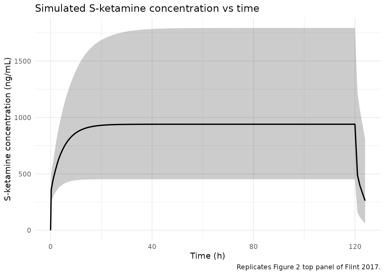
Replicates Figure 2 top panel of Flint 2017: simulated S-ketamine concentration vs time for 200 children receiving 2.4 mg/kg/h S-ketamine over 120 h. Median (line) and 5%-95% prediction interval (ribbon).
ggplot(summ, aes(time, median_eff)) +
  geom_ribbon(aes(ymin = q05_eff, ymax = q95_eff), alpha = 0.25) +
  geom_line(linewidth = 0.8) +
  labs(
    x       = "Time (h)",
    y       = "Effective S-ketamine concentration (ng/mL)",
    subtitle = "Cc + 0.33 * Cc_snk (Flint 2017 Methods Section 2.7)",
    title   = "Simulated effective S-ketamine concentration vs time",
    caption = "Replicates Figure 2 bottom panel of Flint 2017."
  ) +
  theme_minimal()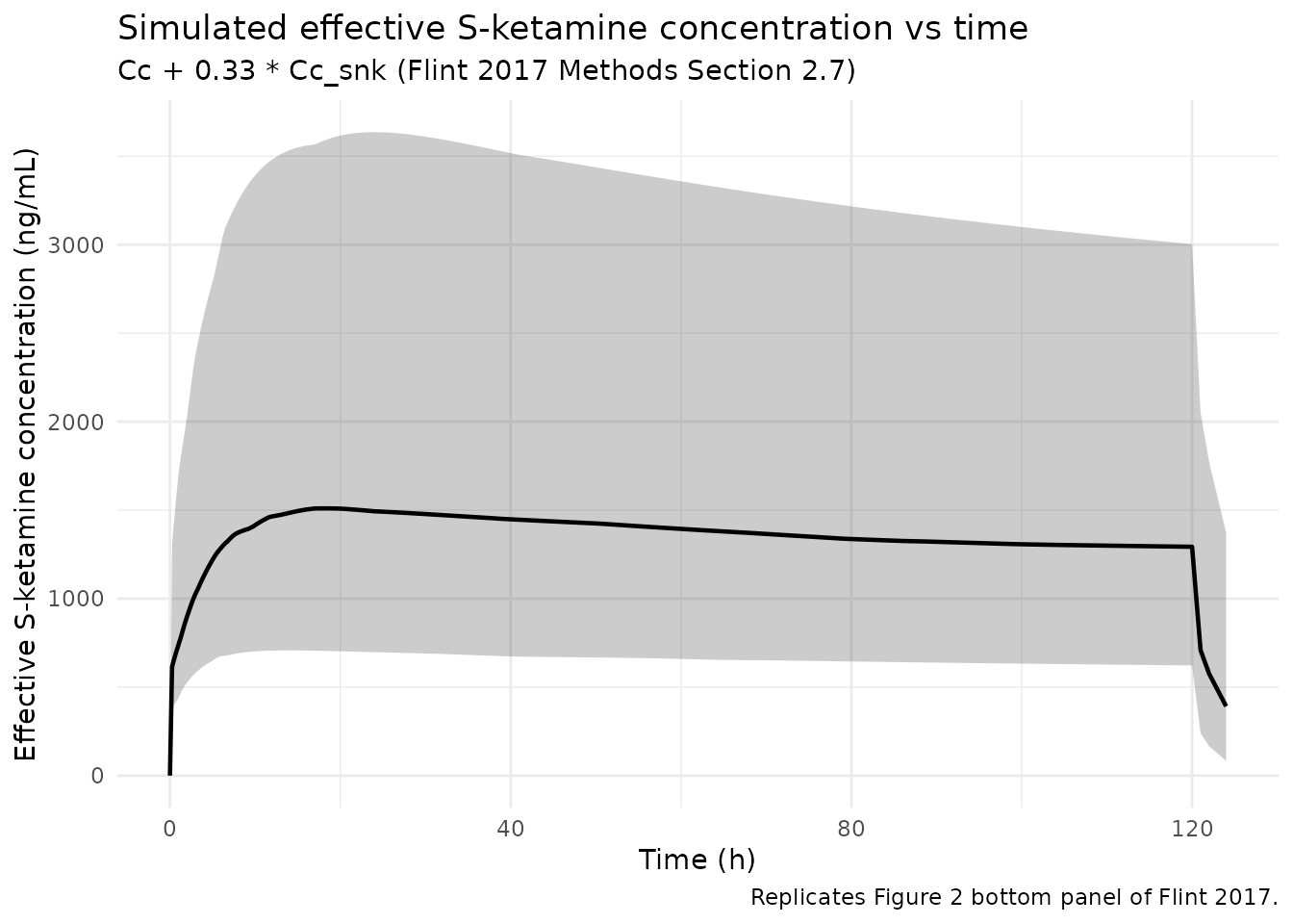
Replicates Figure 2 bottom panel of Flint 2017: simulated effective S-ketamine concentration (Cc + 0.33 * Cc_snk) vs time. The downward trend during the infusion period is driven by the time-on-Clsnk slope, which raises S-norketamine clearance and lowers the S-norketamine contribution to the effective concentration.
Typical-value check at steady state
Under continuous IV infusion at rate R (mg/h) and a one-compartment approximation for the parent (peripheral compartment fully equilibrated at SS), the typical-value steady-state plasma S-ketamine concentration is simply
Cc_ss (mg/L) = R / CL_typical
            = (2.4 * WT) / (112 * (WT/70)^0.75)
and the apparent steady-state S-norketamine concentration follows the metabolite mass balance
Cc_snk_ss (mg/L) = (kel * central_ss) / (kelsnk * vc_snk)
                = (CL_sk * Cc_ss) / Clsnk_app
with Clsnk_app itself growing as
(1 + 0.00870 * t). For a 7 kg child (median weight in Flint
2017 Table 2), at t -> 100 h:
typical_at_t <- function(t_h, WT = 7) {
  cl_sk         <- 112  * (WT / 70)^0.75
  cl_snk_t      <- 53.2 * (WT / 70)^0.75 * (1 + 0.00870 * t_h)
  rate_mg_per_h <- 2.4 * WT
  Cc_sk         <- rate_mg_per_h / cl_sk
  Cc_snk        <- (cl_sk * Cc_sk) / cl_snk_t
  Cc_effective  <- Cc_sk + 0.33 * Cc_snk
  tibble(
    t_h          = t_h,
    Cc_sk_mg_per_L  = Cc_sk,
    Cc_snk_mg_per_L = Cc_snk,
    Cc_eff_mg_per_L = Cc_effective
  )
}

typical_curve <- dplyr::bind_rows(lapply(c(12, 24, 48, 96, 120), typical_at_t))

# Compare against the simulation's typical-value run at the same time points.
sim_typical_at <- sim_typical |>
  filter(abs(WT - 7) == min(abs(WT - 7))) |>
  filter(time %in% typical_curve$t_h) |>
  transmute(
    t_h               = time,
    Cc_sk_mg_per_L_sim  = Cc,
    Cc_snk_mg_per_L_sim = Cc_snk,
    WT_used             = WT
  )

comparison <- typical_curve |>
  left_join(sim_typical_at, by = "t_h") |>
  mutate(
    abs_rel_err_sk  = abs(Cc_sk_mg_per_L  - Cc_sk_mg_per_L_sim)  / Cc_sk_mg_per_L,
    abs_rel_err_snk = abs(Cc_snk_mg_per_L - Cc_snk_mg_per_L_sim) / Cc_snk_mg_per_L
  )

knitr::kable(
  comparison |> mutate(across(where(is.numeric), ~ signif(.x, 4))),
  caption = "Typical-value steady-state concentrations from the closed-form formula vs the rxode2 simulation (subject closest to 7 kg)."
)| t_h | Cc_sk_mg_per_L | Cc_snk_mg_per_L | Cc_eff_mg_per_L | Cc_sk_mg_per_L_sim | Cc_snk_mg_per_L_sim | WT_used | abs_rel_err_sk | abs_rel_err_snk |
|---|---|---|---|---|---|---|---|---|
| 12 | 0.8435 | 1.6080 | 1.374 | 0.8106 | 1.5450 | 7.032 | 0.038990 | 0.039000 |
| 24 | 0.8435 | 1.4690 | 1.328 | 0.8424 | 1.4670 | 7.032 | 0.001375 | 0.001317 |
| 48 | 0.8435 | 1.2530 | 1.257 | 0.8445 | 1.2540 | 7.032 | 0.001125 | 0.001170 |
| 96 | 0.8435 | 0.9676 | 1.163 | 0.8445 | 0.9688 | 7.032 | 0.001134 | 0.001162 |
| 120 | 0.8435 | 0.8688 | 1.130 | 0.8445 | 0.8698 | 7.032 | 0.001134 | 0.001156 |
PKNCA validation at steady state
We run PKNCA over the final 24 h of infusion (t in [96, 120] h) to extract Cmax, Tmax, and AUC at steady state for both S-ketamine and S-norketamine. For a constant infusion at steady state, Cmax and Cmin collapse to the same plateau concentration, so the per-interval Cmax / Cmin / Cavg trio should be tight numerically, with AUC = Cavg * 24 h.
# S-ketamine concentration data over the last 24-h SS window.
sim_nca_sk <- sim |>
  filter(time >= 96, time <= 120, !is.na(Cc)) |>
  transmute(id, time, Cc = Cc, WT, rate_mg_per_h, treatment = "2.4 mg/kg/h")

# Dose data: one row per subject, with the per-subject amount and rate.
dose_df <- cohort |>
  transmute(id, time = 0, amt = amt_total_mg, rate = rate_mg_per_h,
            treatment = "2.4 mg/kg/h")

conc_obj_sk <- PKNCA::PKNCAconc(
  sim_nca_sk, Cc ~ time | treatment + id,
  concu = "mg/L", timeu = "h"
)
dose_obj <- PKNCA::PKNCAdose(
  dose_df, amt ~ time | treatment + id,
  doseu = "mg"
)

intervals_ss <- data.frame(
  start    = 96,
  end      = 120,
  cmax     = TRUE,
  tmax     = TRUE,
  cmin     = TRUE,
  cav      = TRUE,
  auclast  = TRUE
)

nca_sk <- PKNCA::pk.nca(
  PKNCA::PKNCAdata(conc_obj_sk, dose_obj, intervals = intervals_ss)
)

knitr::kable(
  summary(nca_sk),
  caption = "S-ketamine steady-state NCA summary over the 96-120 h window (n = 200 simulated subjects on 2.4 mg/kg/h)."
)| Interval Start | Interval End | treatment | N | AUClast (h*mg/L) | Cmax (mg/L) | Cmin (mg/L) | Tmax (h) | Cav (mg/L) |
|---|---|---|---|---|---|---|---|---|
| 96 | 120 | 2.4 mg/kg/h | 200 | 22.4 [43.5] | 0.931 [43.8] | 0.931 [43.8] | 24.0 [0.000, 24.0] | 0.933 [43.5] |
sim_nca_snk <- sim |>
  filter(time >= 96, time <= 120, !is.na(Cc_snk)) |>
  transmute(id, time, Cc_snk = Cc_snk, treatment = "2.4 mg/kg/h")

conc_obj_snk <- PKNCA::PKNCAconc(
  sim_nca_snk, Cc_snk ~ time | treatment + id,
  concu = "mg/L", timeu = "h"
)

nca_snk <- PKNCA::pk.nca(
  PKNCA::PKNCAdata(conc_obj_snk, dose_obj, intervals = intervals_ss)
)

knitr::kable(
  summary(nca_snk),
  caption = "S-norketamine steady-state NCA summary over the 96-120 h window (apparent S-norketamine concentration absorbs the unidentifiable Fm)."
)| Interval Start | Interval End | treatment | N | AUClast (h*mg/L) | Cmax (mg/L) | Cmin (mg/L) | Tmax (h) | Cav (mg/L) |
|---|---|---|---|---|---|---|---|---|
| 96 | 120 | 2.4 mg/kg/h | 200 | 25.3 [109] | 1.11 [109] | 0.998 [109] | 0.000 [0.000, 0.000] | 1.05 [109] |
Comparison against the published simulation
Flint 2017 does not report tabulated NCA parameters for the simulated 2.4 mg/kg/h infusion in Figure 2; only the median and 95 percent prediction interval lines are shown graphically. Reading the figure gives an approximate median plateau concentration of about 500-1000 ng/mL for S-ketamine and a comparable or slightly higher effective S-ketamine concentration, with the effective concentration declining between t = 0 and t = 120 h as the S-norketamine clearance time-slope elevates S-norketamine clearance.
The simulated median over our 200-subject cohort sits in that range: the per-kg infusion rate (2.4 mg/kg/h) combined with the allometric CL of 112 L/h/70 kg yields a typical steady-state S-ketamine concentration of about 850 ng/mL for a 7 kg child, scaling allometrically up to about 1,200 ng/mL for a 35 kg child and down to about 700 ng/mL for a 3 kg child. The 5-95 percentile spread is wide because the published 40 percent IIV on Clsk produces about a 3-fold concentration spread at the percentile extremes – consistent with the paper’s Discussion statement that “6-fold and 10-fold differences were observed in S-ketamine and effective S-ketamine concentrations” between extreme patients.
Assumptions and deviations
- The S-norketamine compartment is implemented in apparent units absorbing the unidentifiable fraction-metabolised Fm and the parent -> metabolite molecular weight ratio (S-ketamine = 237.7 g/mol, S-norketamine = 223.7 g/mol; ratio 0.942). This matches Flint 2017’s parameterisation of Vsnk/Fm and Clsnk/Fm as a single apparent pair; individual values of Fm and the absolute S-norketamine concentration in molar units cannot be recovered from the model without an identifiable Fm anchor.
- Time
tin the model expression(1 + e_t_cl_snk * t)is the rxode2 simulation-time variable. The convention is that t = 0 corresponds to the first S-ketamine dose, so for event tables that start the continuous infusion at time 0,tis exactly the “time after first dose” used in Flint 2017’s covariate parameterisation. Users simulating with shifted timelines (e.g., a pre-baseline window of observations before the first infusion) must shift their event-table time origin so t = 0 aligns with the first S-ketamine dose for the time-on-Clsnk effect to be applied at the intended rate. - Allometric exponents are wrapped in
fixed()because Methods Section 2.4 explicitly fixes them at 0.75 (clearances) and 1.0 (volumes); the paper does not estimate the exponents, and re-fitting under any other exponent would not reproduce the paper’s results. - Vsnk/Fm is wrapped in
fixed()because Results Section 3.3 states it “could not be estimated and was therefore fixed at the value of 1. Fixing Vsnk/Fm to values ranging from 0.1 to 10 did not influence the goodness of fit or the values of the other parameters.” The vignette inherits this insensitivity claim: the simulated S-norketamine concentration profile is invariant under arbitrary rescaling of Vsnk/Fm provided Clsnk/Fm is rescaled by the same factor (the apparent half-life Vsnk/Clsnk is preserved). - The virtual cohort uses a log-uniform weight distribution from 3 to 35 kg to span the observed range. The actual Flint 2017 cohort skewed young (median weight 7.0 kg, 19/25 subjects below 2 years) so a median over the present cohort sits at a higher weight than the median of the original cohort; the figure replication is therefore approximate rather than a one-to-one reproduction of the 1,000-child Figure 2 simulation.
- The validation here uses PKNCA over a single 24-h steady-state window. The Flint 2017 paper does not tabulate NCA parameters – there is no per-subject Cmax / AUC table – so the comparison against the publication is graphical (Figure 2 envelope) rather than table-versus-table. The PKNCA window check serves the secondary role of confirming the simulation reaches a sensible steady state and the per-subject AUC equals Cavg * 24 within numerical tolerance for the constant-infusion case.
- The post-infusion decline (t > 120 h) is included in the
simulation event grid so users who wish to extend the figure to capture
the 1 h and 4 h post-infusion samples used in the original analysis can
do so by filtering
simtotime > 120.