Dexamethasone, erythrocyte-encapsulated (Ozdin 2025)
Source:vignettes/articles/Ozdin_2025_dexamethasone.Rmd
Ozdin_2025_dexamethasone.RmdModel and source
mod <- rxode2::rxode(readModelDb("Ozdin_2025_dexamethasone"))- Citation: Ozdin D, Kheibarshekan L, Mambrini G, Tremblay PO. Population Pharmacokinetic Modeling and Pediatric Exposure of Dexamethasone Sodium Phosphate Encapsulated in Erythrocytes (eDSP) Administered Monthly for Treatment of Neurological Symptoms of Patients With Ataxia Telangiectasia. CPT Pharmacometrics Syst Pharmacol. 2025;14(11):1882-1892. doi:10.1002/psp4.70103.
- Description: Two-compartment population PK model with linear elimination for dexamethasone released from dexamethasone sodium phosphate (DSP) encapsulated in autologous erythrocytes (eDSP, the EryDex System) given as a monthly intravenous infusion, in 133 pooled subjects: 18 healthy adults from a phase 1 single-dose study (NCT01925859) and 115 patients with ataxia telangiectasia (109 pediatric, 6 adult) from the phase 3 ATTeST study (NCT02770807). Dexamethasone is released from the infused red blood cells over 20-30 days, so eDSP behaves as a sustained-release depot; the authors evaluated depot, dual-absorption, Michaelis-Menten and semi-physiological release structures and retained the simpler two-compartment disposition model, which estimates systemic exposure adequately without reproducing the underlying triphasic release. Body weight scales clearances (exponent fixed to 0.75 on CL and Q) and volumes (exponent fixed to 1 on V1 and V2) about a 70 kg reference. Clearance is about 10 percent lower in patients with ataxia telangiectasia than in healthy adults. Between-subject variability is carried on CL and V1 only. Combined proportional plus additive residual error is stratified between the phase 1 healthy cohort and the phase 3 patient cohort.
- Article: https://doi.org/10.1002/psp4.70103
- Supplement (Appendix S1, contains Tables S1-S4, Figures S1-S10 and the final NONMEM control stream): https://doi.org/10.1002/psp4.70103
The EryDex System (EDS) loads dexamethasone sodium phosphate (DSP) into the patient’s own erythrocytes ex vivo. After the loaded cells are infused back, resident phosphatases dephosphorylate DSP to dexamethasone, which then diffuses passively across the red-cell membrane over a period of weeks. eDSP therefore behaves as a sustained-release depot even though it is given intravenously.
The authors evaluated depot, dual-absorption, Michaelis-Menten-absorption and semi-physiological release structures (supplement Figures S3 and S4) and retained none of them: adding phase 3 data to the semi-physiological model drove the inter-compartmental clearance to an implausibly low value and its between-subject variability could not be estimated, which the authors ascribe to over-parameterisation. The packaged model is therefore the plain two-compartment disposition model with linear elimination that the paper selected (Results section 3.3, supplement Figure S2), which the authors themselves describe as adequate for systemic exposure but not a mechanistic description of red-cell release.
Population
The pooled analysis dataset contains 133 subjects and 1719 dexamethasone plasma concentrations from two studies (Ozdin 2025 Table 1, Table S1):
- Phase 1 (NCT01925859): 18 healthy adults, single intravenous eDSP infusion over approximately 10 min, dense sampling from 15 min out to day 42. Nine subjects received the half-low dose (approximately 2.5-5 mg DSP encapsulated) and nine the high dose (approximately 14-22 mg).
- Phase 3 ATTeST (NCT02770807): 115 patients with ataxia telangiectasia (109 pediatric, 6 adult), monthly intravenous eDSP infusions over approximately 40 min for one year, sparse sampling (pre-dose, 1 h and 4 h post-infusion on day 1, 24 h, and day 15 after the first dose; trough and peak around doses 2-5; trough only before dose 6). Fifty-eight patients received the low dose (mean 8.3 mg) and 57 the high dose (mean 17.4 mg).
Overall the cohort was 47% female and 57% White / 43% African American or Black, with a median age of 10.0 years (range 5.00-55.0) and a median weight of 25.0 kg (range 15.1-95.7). By age group there were 24 adults (18 healthy from phase 1 plus 6 patients from phase 3), 44 children aged 10 to under 17 years, 64 aged 6 to under 10 years, and a single subject aged 2 to under 6 years. The paper repeatedly cautions against extrapolating to the youngest band for that reason, and no maturation function was incorporated.
The same information is available programmatically:
str(readModelDb("Ozdin_2025_dexamethasone")()$population)
#> List of 13
#>  $ species       : chr "human"
#>  $ n_subjects    : num 133
#>  $ n_studies     : num 2
#>  $ age_range     : chr "5.00-55.0 years"
#>  $ age_median    : chr "10.0 years"
#>  $ weight_range  : chr "15.1-95.7 kg"
#>  $ weight_median : chr "25.0 kg"
#>  $ sex_female_pct: num 47
#>  $ race_ethnicity: Named num [1:2] 57 43
#>   ..- attr(*, "names")= chr [1:2] "White" "Black"
#>  $ disease_state : chr "ataxia telangiectasia (115 subjects, phase 3 ATTeST NCT02770807) and healthy adults (18 subjects, phase 1 NCT01925859)"
#>  $ dose_range    : chr "4.2, 8.3 and 17.4 mg DSP encapsulated in red blood cells per intravenous infusion; single dose over approximate"| __truncated__
#>  $ regions       : chr "international, multi-center (phase 3); single-center (phase 1)"
#>  $ notes         : chr "Baseline demographics from Ozdin 2025 Table 1. Age groups: adults n = 24 (18 healthy from phase 1 plus 6 patien"| __truncated__
Source trace
Every ini() value carries an in-file comment naming its
source location in
inst/modeldb/specificDrugs/Ozdin_2025_dexamethasone.R. The
table collects them for review. “Table 2” is the final population PK
parameter table of the main article; “control stream” is the
Final PK Model - NONMEM File listing at the end of
supplement Appendix S1.
| Equation / parameter | Value | Source location |
|---|---|---|
lcl |
log(20.8 * 0.899) = log(18.70) |
Table 2, Clearance CL (L/h) = 20.8 (RSE 8%), shifted to
the patient reference by the Table 2 Patient effect on CL
factor 0.899 |
lvc |
log(122) |
Table 2, Central volume V1 (L) = 122 (RSE 9%) |
lq |
log(0.358) |
Table 2, Inter-compartmental clearance Q (L/h) = 0.358
(RSE 13%) |
lvp |
log(16.8) |
Table 2, Peripheral volume V2 (L) = 16.8 (RSE 9%) |
e_wt_cl_q |
fixed(0.75) |
Table 2, Weight effect on CL and
Weight effect on Q, both “0.75 FIXED”; control stream
(WTBL/70)**0.75
|
e_wt_vc_vp |
fixed(1) |
Table 2, Weight effect on V1 and
Weight effect on V2, both “1 FIXED”; control stream
(WTBL/70)**1
|
e_dis_healthy_cl |
1 / 0.899 = 1.112 |
Table 2, Patient effect on CL -> * theta_PTNT =
0.899 (RSE 10%); control stream THETA(9)**PTNT. Reciprocal
because the canonical column is DIS_HEALTHY = 1 - PTNT
|
etalcl |
log(1 + 0.414^2) = 0.1582 |
Table 2, ETA_CL = 41.4% CV (RSE 51%, shrinkage
26%) |
etalvc |
log(1 + 0.707^2) = 0.4054 |
Table 2, ETA_V1 = 70.7% CV (RSE 21%, shrinkage 7%) |
| no IIV on Q, V2 | – | Control stream $OMEGA 0 FIX for Q and V2; Results
section 3.3 (“Inter-individual variability was introduced only on CL and
V1”) |
propSdHealthy |
0.181 | Table 2, Proportional Error (%)-Phase 1 = 18.1% (RSE
10%) |
addSdHealthy |
0.0013 | Table 2, Additive error (ng/mL)-Phase 1 = 0.0013 (RSE
18%) |
propSdPatient |
0.295 | Table 2, Proportional Error (%)-Phase 3 = 29.5% (RSE
23%) |
addSdPatient |
24.3 | Table 2, Additive error (ng/mL)-Phase 3 = 24.3 (RSE
58%) |
d/dt(central), d/dt(peripheral1)
|
n/a | Supplement Figure S2 (structural schematic); control stream
$SUBROUTINE ADVAN3 TRANS4
|
cl, vc, q, vp
covariate forms |
n/a | Control stream $PK block:
TVCL=THETA(1)*(WTBL/70)**0.75 * THETA(9)**PTNT,
TVV1=THETA(2)*(WTBL/70)**1,
TVQ=THETA(3)*(WTBL/70)**0.75,
TVV2=THETA(4)*(WTBL/70)**1
|
Cc ~ prop(propSd) + add(addSd) |
n/a | Control stream $ERROR:
W = (PROPn*PROPn*IPRED*IPRED + ADDn*ADDn)**0.5,
Y = IPRED + W*EPS(1), $SIGMA 1 FIX
|
Cc <- 1000 * central / vc |
n/a | Control stream S1=V1 with dose amounts in ug;
re-expressed here with dose in mg (the unit the paper reports doses in)
so the 1000 converts mg/L to the ng/mL of Table 2, Table 3 and Tables
S1-S4 |
Two source readings that had to be resolved
Residual error keyed on study phase. The control
stream branches the residual error on PHAS (1 or 3) while
the clearance effect uses PTNT (0 = healthy, 1 = patient).
Because every phase 1 subject is a healthy adult and every phase 3
subject is an ataxia-telangiectasia patient (Methods section 2.1, Table
1), the two columns partition the pooled dataset identically. Both are
therefore carried on the single canonical covariate
DIS_HEALTHY = 1 - PTNT.
Scale of the reported between-subject variability.
Table 2 gives BSV as “41.4%” and “70.7%” under the heading
Between Subject Variability (CV%) without stating whether
these are the exact log-normal CV
(100 * sqrt(exp(omega^2) - 1)) or the approximation
100 * sqrt(omega^2). The two readings imply materially
different variances for V1 (0.4054 versus 0.4998). The model file
encodes the exact-CV reading, on the following evidence:
-
Decisive. It reproduces the control stream’s
$OMEGA(2,2)starting value:log(1 + 0.707^2) = 0.4054versus the listed 0.404706, a 0.2% difference, where the alternative reading would be 23% away. The phase 3 residual-error starting values behave the same way (PROP20.296021 versus the Table 2 final 0.295;ADD224.2317 versus 24.3), so the control stream’s initial estimates are evidently a previous run’s near-converged values, which makes that agreement meaningful rather than coincidental. -
Supporting. It is the convention used throughout
nlmixr2lib. - Corroborating but not decisive. It reproduces the simulated Cmax spread of Table 3 somewhat better. The check is run explicitly below, where the margin between the two readings turns out to be only one to two Monte Carlo standard errors at the cohort sizes this vignette is allowed to use – so it points the same way in all three age bands, but would not settle the question on its own.
Model structure and typical-value behaviour
Before simulating cohorts, confirm the deterministic behaviour of the packaged model against quantities that can be derived in closed form.
tv <- rxode2::zeroRe(mod)
#> Warning: No sigma parameters in the model

wt_ref  <- 50.7   # median weight, 10-<17 years (Table 3)
dose_ld <- 8.3    # low dose, mg DSP encapsulated (Methods section 2.6)
tau     <- 720    # monthly dosing interval, h
inf_dur <- 40 / 60  # phase 3 infusion duration, approximately 40 min

# Closed-form clearance and AUCinf for an AT patient at the reference weight.
cl_cf   <- 20.8 * 0.899 * (wt_ref / 70)^0.75
auc_cf  <- dose_ld * 1000 / cl_cf

ev_tv <- rxode2::et(time = 0, amt = dose_ld, dur = inf_dur, cmt = "central") |>
  rxode2::et(sort(unique(c(seq(0, 1, by = 0.05), inf_dur,
                           seq(1.5, 24, by = 0.5),
                           seq(28, tau, by = 2)))), cmt = "central") |>
  as.data.frame() |>
  mutate(WT = wt_ref, DIS_HEALTHY = 0)

sim_tv <- rxode2::rxSolve(tv, ev_tv, returnType = "data.frame")
#> ℹ omega/sigma items treated as zero: 'etalcl', 'etalvc'

auc_sim <- sum(diff(sim_tv$time) *
                 (head(sim_tv$Cc, -1) + tail(sim_tv$Cc, -1)) / 2)
# Analytic terminal (beta) half-life from the eigenvalues of the two-compartment
# system at the reference weight.
vc_r <- 122   * (wt_ref / 70)
q_r  <- 0.358 * (wt_ref / 70)^0.75
vp_r <- 16.8  * (wt_ref / 70)
k10 <- cl_cf / vc_r; k12 <- q_r / vc_r; k21 <- q_r / vp_r
beta_r <- ((k10 + k12 + k21) - sqrt((k10 + k12 + k21)^2 - 4 * k10 * k21)) / 2
alpha_r <- (k10 + k12 + k21) - beta_r

tibble::tibble(
  Quantity = c("CL (L/h)", "AUC0-inf = dose/CL (ng*h/mL)",
               "AUC0-720 simulated (ng*h/mL)", "Cmax simulated (ng/mL)",
               "Tmax simulated (h)", "Distribution t1/2 (h)",
               "Terminal t1/2 (h)", "Terminal t1/2 (days)"),
  Value = c(cl_cf, auc_cf, auc_sim, max(sim_tv$Cc),
            sim_tv$time[which.max(sim_tv$Cc)],
            log(2) / alpha_r, log(2) / beta_r, log(2) / beta_r / 24)
) |>
  knitr::kable(digits = 3,
caption = "Typical-value behaviour at 50.7 kg, low dose (8.3 mg).")| Quantity | Value |
|---|---|
| CL (L/h) | 14.681 |
| AUC0-inf = dose/CL (ng*h/mL) | 565.357 |
| AUC0-720 simulated (ng*h/mL) | 565.880 |
| Cmax simulated (ng/mL) | 88.824 |
| Tmax simulated (h) | 0.667 |
| Distribution t1/2 (h) | 4.082 |
| Terminal t1/2 (h) | 30.672 |
| Terminal t1/2 (days) | 1.278 |
Three checks pass here. AUC0-720 from the ODE equals the
closed-form dose / CL identity, which simultaneously gates
the ODE system, the dose encoding, the 1000 * unit
conversion and the observation grid. The simulated Tmax lands at the end
of the 40-min infusion, matching the paper’s statement that Cmax “is
expected to occur at the end of eDSP infusion (approximately 0.67 h)”.
And the simulated Cmax of about 88 ng/mL is within 1% of the median 88.1
ng/mL that Ozdin 2025 Table 3 reports for the same age group and
dose.
Virtual cohort
Individual data are not public. The cohort below mirrors the Monte
Carlo population of Ozdin 2025 Methods section 2.6: three pediatric age
bands crossed with the three dose levels, all coded as
ataxia-telangiectasia patients (DIS_HEALTHY = 0). The paper
drew weights from CDC growth charts with a GAMLSS fit and used 1000
subjects per age band; here each of the nine arms uses 100 subjects, and
weights are drawn from a log-normal matched to the median and CV that
Table 3 reports for each band, truncated to the reported minimum and
maximum.
set.seed(20250311)

n_arm <- 100

age_bands <- tibble::tribble(
  ~agegrp,   ~wt_median, ~wt_cv, ~wt_min, ~wt_max,
  "2-<6 y",        16.3,  0.208,    10.4,    31.9,
  "6-<10 y",       28.1,  0.264,    16.3,    65.6,
  "10-<17 y",      50.7,  0.213,    24.6,    69.9
)

dose_levels <- tibble::tribble(
  ~dose,          ~amt,
  "H-LD 4.2 mg",   4.2,
  "LD 8.3 mg",     8.3,
  "HD 17.4 mg",   17.4
)

# Draw n truncated log-normal weights matched to a median and CV.
sample_weights <- function(n, wt_median, wt_cv, wt_min, wt_max) {
  sdlog <- sqrt(log(1 + wt_cv^2))
  out <- numeric(0)
  while (length(out) < n) {
    draw <- stats::rlnorm(4 * n, log(wt_median), sdlog)
    out <- c(out, draw[draw >= wt_min & draw <= wt_max])
  }
  out[seq_len(n)]
}

n_doses    <- 6                                  # monthly infusions over 6 months
dose_times <- seq(0, by = tau, length.out = n_doses)

# Dense sampling in the first and sixth intervals (the two the paper tabulates),
# daily sampling in between. 0.05 h spacing in the first hour after each dose
# resolves the end-of-infusion peak, as in Methods section 2.6.
grid_dense  <- sort(unique(c(seq(0, 1, by = 0.05), inf_dur,
                             seq(1.5, 24, by = 0.5), seq(28, tau - 4, by = 4))))
grid_coarse <- seq(0, tau - 24, by = 24)
obs_times   <- sort(unique(c(
  grid_dense,
  dose_times[n_doses] + grid_dense,
  as.numeric(outer(dose_times[2:(n_doses - 1)], grid_coarse, "+"))
)))

make_arm <- function(agegrp, wt_median, wt_cv, wt_min, wt_max,
                     dose, amt, id_offset) {
  wt <- sample_weights(n_arm, wt_median, wt_cv, wt_min, wt_max)
  ev <- rxode2::et(time = dose_times, amt = amt, dur = inf_dur, cmt = "central") |>
    rxode2::et(obs_times, cmt = "central") |>
    rxode2::et(id = seq_len(n_arm)) |>
    as.data.frame()
  ev$WT          <- wt[ev$id]
  ev$id          <- ev$id + id_offset
  ev$DIS_HEALTHY <- 0
  ev$agegrp      <- agegrp
  ev$dose        <- dose
  ev
}

arms <- tidyr::crossing(age_bands, dose_levels) |>
  mutate(
    agegrp = factor(agegrp, levels = age_bands$agegrp),
    dose   = factor(dose,   levels = dose_levels$dose)
  ) |>
  arrange(agegrp, dose) |>
  mutate(id_offset = (row_number() - 1L) * n_arm)

events <- do.call(
  rbind,
  lapply(seq_len(nrow(arms)), function(i) {
    make_arm(as.character(arms$agegrp[i]), arms$wt_median[i], arms$wt_cv[i],
             arms$wt_min[i], arms$wt_max[i], as.character(arms$dose[i]),
             arms$amt[i], arms$id_offset[i])
  })
)
events$agegrp <- factor(events$agegrp, levels = age_bands$agegrp)
events$dose   <- factor(events$dose,   levels = dose_levels$dose)

# IDs must be disjoint across arms or rxSolve silently merges subjects.
stopifnot(length(unique(events$id)) == nrow(arms) * n_arm)
stopifnot(!anyDuplicated(events[events$evid == 0, c("id", "time")]))

events |>
  filter(evid == 1, time == 0) |>
  group_by(agegrp) |>
  summarise(n = n() / nrow(dose_levels),
            `Weight mean (kg)` = mean(WT[dose == dose_levels$dose[1]]),
            `Weight CV%` = 100 * sd(WT[dose == dose_levels$dose[1]]) /
              mean(WT[dose == dose_levels$dose[1]]),
            `Weight median (kg)` = median(WT[dose == dose_levels$dose[1]]),
            .groups = "drop") |>
  rename("Age band" = agegrp, "N per dose arm" = n) |>
  knitr::kable(digits = 1,
caption = "Simulated weight distributions, for comparison with the Weight rows of Ozdin 2025 Table 3 (means 16.8 / 29.5 / 50.3 kg, CV 20.8 / 26.4 / 21.3%, medians 16.3 / 28.1 / 50.7 kg).")| Age band | N per dose arm | Weight mean (kg) | Weight CV% | Weight median (kg) |
|---|---|---|---|---|
| 2-<6 y | 100 | 17.4 | 20.4 | 16.8 |
| 6-<10 y | 100 | 28.3 | 27.0 | 27.0 |
| 10-<17 y | 100 | 49.8 | 20.3 | 48.4 |
Simulation
sim <- rxode2::rxSolve(mod, events = events, keep = c("agegrp", "dose", "WT"),
                       atol = 1e-12, rtol = 1e-10)

# Deep-tail round-off guard. By 700 h post-dose the model predicts
# concentrations around 1e-7 ng/mL, seven orders of magnitude below the assay
# LLOQ of 0.5 ng/mL (Methods section 2.1); at that scale the solver can return
# values a few times 1e-11 below zero, which PKNCA would turn into NA and which
# would drop out of a log-scale plot. Clamp them at zero.
sim <- sim |>
  mutate(Cc = pmax(Cc, 0),
         agegrp = factor(as.character(agegrp), levels = age_bands$agegrp),
         dose   = factor(as.character(dose),   levels = dose_levels$dose),
         dose_index = pmin(floor(time / tau) + 1, n_doses),
         t_after_dose = time - (dose_index - 1) * tau)
Replicate published figures
# Replicates Figure S9 of Ozdin 2025: simulated dexamethasone profiles over the
# month after the FIRST dose, by pediatric age band and dose level.
sim |>
  filter(dose_index == 1, Cc > 0) |>
  group_by(agegrp, dose, t_after_dose) |>
  summarise(Q05 = quantile(Cc, 0.05), Q50 = median(Cc), Q95 = quantile(Cc, 0.95),
            .groups = "drop") |>
  ggplot(aes(t_after_dose / 24, Q50, colour = dose, fill = dose)) +
  geom_ribbon(aes(ymin = Q05, ymax = Q95), alpha = 0.2, colour = NA) +
  geom_line() +
  geom_hline(yintercept = 0.5, linetype = "dashed", linewidth = 0.3) +
  facet_wrap(~agegrp) +
  scale_y_log10() +
  labs(x = "Time after first dose (days)", y = "Dexamethasone (ng/mL)",
       colour = "Dose", fill = "Dose",
       title = "Figure S9 - simulated single-dose profiles",
       caption = paste("Replicates Figure S9 of Ozdin 2025. Median with 5th-95th",
                       "percentile band. Dashed line = assay LLOQ 0.5 ng/mL.")) +
  theme(legend.position = "bottom")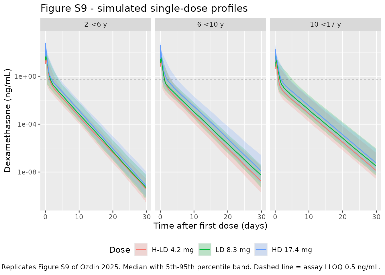
# Replicates Figure S10 of Ozdin 2025: the same profiles over the month
# following the SIXTH monthly dose.
sim |>
  filter(dose_index == n_doses, Cc > 0) |>
  group_by(agegrp, dose, t_after_dose) |>
  summarise(Q05 = quantile(Cc, 0.05), Q50 = median(Cc), Q95 = quantile(Cc, 0.95),
            .groups = "drop") |>
  ggplot(aes(t_after_dose / 24, Q50, colour = dose, fill = dose)) +
  geom_ribbon(aes(ymin = Q05, ymax = Q95), alpha = 0.2, colour = NA) +
  geom_line() +
  geom_hline(yintercept = 0.5, linetype = "dashed", linewidth = 0.3) +
  facet_wrap(~agegrp) +
  scale_y_log10() +
  labs(x = "Time after sixth dose (days)", y = "Dexamethasone (ng/mL)",
       colour = "Dose", fill = "Dose",
       title = "Figure S10 - simulated sixth-dose profiles",
       caption = paste("Replicates Figure S10 of Ozdin 2025. Visually identical",
                       "to Figure S9, i.e. no accumulation.")) +
  theme(legend.position = "bottom")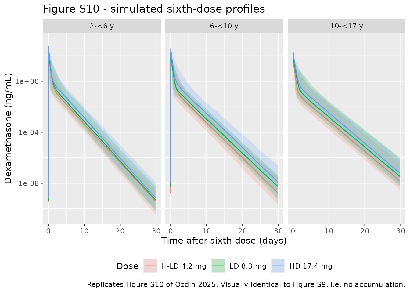
PKNCA validation
Exposure metrics are computed with PKNCA over two windows: the first
monthly interval (Ozdin 2025 Table 3) and the sixth (Table S3). Both
tables report “AUC over one month”, so auclast on a
[dose, dose + 720 h] interval is the matching
parameter.
# PKNCA reserves "dose" as one of its standardized column names, so the dose
# group is carried as `dosegrp` from here on.
sim_nca <- sim |>
  filter(!is.na(Cc)) |>
  select(id, time, Cc, agegrp, dosegrp = dose)

# Guarantee a time-zero record per subject so PKNCA can anchor AUC without
# emitting "Requesting an AUC range starting (0) before the first measurement".
sim_nca <- bind_rows(
  sim_nca,
  sim_nca |> distinct(id, agegrp, dosegrp) |> mutate(time = 0, Cc = 0)
) |>
  distinct(id, agegrp, dosegrp, time, .keep_all = TRUE) |>
  arrange(id, time)

conc_obj <- PKNCA::PKNCAconc(sim_nca, Cc ~ time | agegrp + dosegrp + id)

dose_df <- events |>
  filter(evid == 1) |>
  select(id, time, amt, agegrp, dosegrp = dose)

dose_obj <- PKNCA::PKNCAdose(dose_df, amt ~ time | agegrp + dosegrp + id)

intervals <- data.frame(
  start   = c(0, dose_times[n_doses]),
  end     = c(tau, dose_times[n_doses] + tau),
  cmax    = TRUE,
  tmax    = TRUE,
  auclast = TRUE
)

nca_res <- PKNCA::pk.nca(
  PKNCA::PKNCAdata(conc_obj, dose_obj, intervals = intervals)
)

nca_long <- as.data.frame(nca_res) |>
  mutate(window = if_else(start == 0, "First dose", "Sixth dose"))
cl.obs and vz.obs are deliberately not
requested: the concentrations are in ng/mL while the dose amounts are in
mg, so PKNCA would report them a factor of 1000 away from the model’s
L/h and L. The closed-form table above covers those quantities
instead.
Comparison against published exposures - first dose (Table 3)
ncaComparisonTable() aggregates the simulated subjects
by median, so the reference column transcribes the
median values of Ozdin 2025 Table 3 (the table reports
Mean (CV%) above Median [Min, Max] in each
cell). Tmax is not tabulated; the 0.67 h reference is the
end-of-infusion value stated in Results section 3.5 and the
Discussion.
published_first <- tibble::tribble(
  ~agegrp,      ~dosegrp,         ~cmax, ~auclast, ~tmax,
  "2-<6 y",     "H-LD 4.2 mg",   132,      685,  0.67,
  "2-<6 y",     "LD 8.3 mg",     260,     1354,  0.67,
  "2-<6 y",     "HD 17.4 mg",    546,     2838,  0.67,
  "6-<10 y",    "H-LD 4.2 mg",  80.0,      434,  0.67,
  "6-<10 y",    "LD 8.3 mg",     158,      857,  0.67,
  "6-<10 y",    "HD 17.4 mg",    331,     1796,  0.67,
  "10-<17 y",   "H-LD 4.2 mg",  44.6,      292,  0.67,
  "10-<17 y",   "LD 8.3 mg",    88.1,      578,  0.67,
  "10-<17 y",   "HD 17.4 mg",    185,     1211,  0.67
)

cmp_first <- nlmixr2lib::ncaComparisonTable(
  simulated     = nca_long |> filter(window == "First dose"),
  reference     = published_first,
  by            = c("agegrp", "dosegrp"),
  params        = c("cmax", "auclast", "tmax"),
  units         = c(cmax = "ng/mL", auclast = "ng*h/mL", tmax = "h"),
  tolerance_pct = 20
)

knitr::kable(
  cmp_first,
  caption = "Simulated vs. Ozdin 2025 Table 3 medians (single dose). * differs from reference by >20%."
)| NCA parameter | agegrp | dosegrp | Reference | Simulated | % diff |
|---|---|---|---|---|---|
| Cmax (ng/mL) | 2-<6 y | H-LD 4.2 mg | 132 | 126 | -4.2% |
| Cmax (ng/mL) | 2-<6 y | LD 8.3 mg | 260 | 261 | +0.6% |
| Cmax (ng/mL) | 2-<6 y | HD 17.4 mg | 546 | 557 | +2.1% |
| Cmax (ng/mL) | 6-<10 y | H-LD 4.2 mg | 80 | 80.3 | +0.4% |
| Cmax (ng/mL) | 6-<10 y | LD 8.3 mg | 158 | 162 | +2.6% |
| Cmax (ng/mL) | 6-<10 y | HD 17.4 mg | 331 | 365 | +10.3% |
| Cmax (ng/mL) | 10-<17 y | H-LD 4.2 mg | 44.6 | 51.1 | +14.6% |
| Cmax (ng/mL) | 10-<17 y | LD 8.3 mg | 88.1 | 82.3 | -6.5% |
| Cmax (ng/mL) | 10-<17 y | HD 17.4 mg | 185 | 185 | -0.2% |
| Tmax (h) | 2-<6 y | H-LD 4.2 mg | 0.67 | 0.667 | -0.5% |
| Tmax (h) | 2-<6 y | LD 8.3 mg | 0.67 | 0.667 | -0.5% |
| Tmax (h) | 2-<6 y | HD 17.4 mg | 0.67 | 0.667 | -0.5% |
| Tmax (h) | 6-<10 y | H-LD 4.2 mg | 0.67 | 0.667 | -0.5% |
| Tmax (h) | 6-<10 y | LD 8.3 mg | 0.67 | 0.667 | -0.5% |
| Tmax (h) | 6-<10 y | HD 17.4 mg | 0.67 | 0.667 | -0.5% |
| Tmax (h) | 10-<17 y | H-LD 4.2 mg | 0.67 | 0.667 | -0.5% |
| Tmax (h) | 10-<17 y | LD 8.3 mg | 0.67 | 0.667 | -0.5% |
| Tmax (h) | 10-<17 y | HD 17.4 mg | 0.67 | 0.667 | -0.5% |
| AUClast (ng*h/mL) | 2-<6 y | H-LD 4.2 mg | 685 | 675 | -1.4% |
| AUClast (ng*h/mL) | 2-<6 y | LD 8.3 mg | 1350 | 1280 | -5.2% |
| AUClast (ng*h/mL) | 2-<6 y | HD 17.4 mg | 2840 | 2440 | -14.0% |
| AUClast (ng*h/mL) | 6-<10 y | H-LD 4.2 mg | 434 | 472 | +8.6% |
| AUClast (ng*h/mL) | 6-<10 y | LD 8.3 mg | 857 | 834 | -2.7% |
| AUClast (ng*h/mL) | 6-<10 y | HD 17.4 mg | 1800 | 1940 | +8.1% |
| AUClast (ng*h/mL) | 10-<17 y | H-LD 4.2 mg | 292 | 285 | -2.3% |
| AUClast (ng*h/mL) | 10-<17 y | LD 8.3 mg | 578 | 614 | +6.2% |
| AUClast (ng*h/mL) | 10-<17 y | HD 17.4 mg | 1210 | 1210 | -0.3% |
Comparison against published exposures - sixth dose (Table S3)
Table S3 of the supplement reports exposures after the sixth monthly dose. Its numbers are byte-for-byte identical to Table 3, which is the paper’s central finding: once-monthly eDSP produces no accumulation. The same reference values are therefore reused here, and the simulated sixth-dose column is an independent test of that structural claim.
cmp_sixth <- nlmixr2lib::ncaComparisonTable(
  simulated     = nca_long |> filter(window == "Sixth dose"),
  reference     = published_first,
  by            = c("agegrp", "dosegrp"),
  params        = c("cmax", "auclast", "tmax"),
  units         = c(cmax = "ng/mL", auclast = "ng*h/mL", tmax = "h"),
  tolerance_pct = 20
)

knitr::kable(
  cmp_sixth,
  caption = "Simulated vs. Ozdin 2025 Table S3 medians (sixth dose). * differs from reference by >20%."
)| NCA parameter | agegrp | dosegrp | Reference | Simulated | % diff |
|---|---|---|---|---|---|
| Cmax (ng/mL) | 2-<6 y | H-LD 4.2 mg | 132 | 126 | -4.2% |
| Cmax (ng/mL) | 2-<6 y | LD 8.3 mg | 260 | 261 | +0.6% |
| Cmax (ng/mL) | 2-<6 y | HD 17.4 mg | 546 | 557 | +2.1% |
| Cmax (ng/mL) | 6-<10 y | H-LD 4.2 mg | 80 | 80.3 | +0.4% |
| Cmax (ng/mL) | 6-<10 y | LD 8.3 mg | 158 | 162 | +2.6% |
| Cmax (ng/mL) | 6-<10 y | HD 17.4 mg | 331 | 365 | +10.3% |
| Cmax (ng/mL) | 10-<17 y | H-LD 4.2 mg | 44.6 | 51.1 | +14.6% |
| Cmax (ng/mL) | 10-<17 y | LD 8.3 mg | 88.1 | 82.3 | -6.5% |
| Cmax (ng/mL) | 10-<17 y | HD 17.4 mg | 185 | 185 | -0.2% |
| Tmax (h) | 2-<6 y | H-LD 4.2 mg | 0.67 | 0.667 | -0.5% |
| Tmax (h) | 2-<6 y | LD 8.3 mg | 0.67 | 0.667 | -0.5% |
| Tmax (h) | 2-<6 y | HD 17.4 mg | 0.67 | 0.667 | -0.5% |
| Tmax (h) | 6-<10 y | H-LD 4.2 mg | 0.67 | 0.667 | -0.5% |
| Tmax (h) | 6-<10 y | LD 8.3 mg | 0.67 | 0.667 | -0.5% |
| Tmax (h) | 6-<10 y | HD 17.4 mg | 0.67 | 0.667 | -0.5% |
| Tmax (h) | 10-<17 y | H-LD 4.2 mg | 0.67 | 0.667 | -0.5% |
| Tmax (h) | 10-<17 y | LD 8.3 mg | 0.67 | 0.667 | -0.5% |
| Tmax (h) | 10-<17 y | HD 17.4 mg | 0.67 | 0.667 | -0.5% |
| AUClast (ng*h/mL) | 2-<6 y | H-LD 4.2 mg | 685 | 675 | -1.4% |
| AUClast (ng*h/mL) | 2-<6 y | LD 8.3 mg | 1350 | 1280 | -5.2% |
| AUClast (ng*h/mL) | 2-<6 y | HD 17.4 mg | 2840 | 2440 | -14.0% |
| AUClast (ng*h/mL) | 6-<10 y | H-LD 4.2 mg | 434 | 472 | +8.6% |
| AUClast (ng*h/mL) | 6-<10 y | LD 8.3 mg | 857 | 834 | -2.7% |
| AUClast (ng*h/mL) | 6-<10 y | HD 17.4 mg | 1800 | 1940 | +8.1% |
| AUClast (ng*h/mL) | 10-<17 y | H-LD 4.2 mg | 292 | 285 | -2.3% |
| AUClast (ng*h/mL) | 10-<17 y | LD 8.3 mg | 578 | 614 | +6.2% |
| AUClast (ng*h/mL) | 10-<17 y | HD 17.4 mg | 1210 | 1210 | -0.3% |
Accumulation ratio
# Replicates Figure 4 of Ozdin 2025: Cmax and AUC after a single dose versus
# after the sixth monthly dose, by age band and dose level.
nca_long |>
  filter(PPTESTCD %in% c("cmax", "auclast")) |>
  mutate(PPTESTCD = recode(PPTESTCD, cmax = "Cmax (ng/mL)",
                           auclast = "AUC (ng*h/mL)")) |>
  ggplot(aes(dosegrp, PPORRES, fill = window)) +
  geom_boxplot(outlier.shape = NA, position = position_dodge(0.8)) +
  facet_grid(PPTESTCD ~ agegrp, scales = "free_y") +
  scale_y_log10() +
  labs(x = NULL, y = NULL, fill = NULL,
       title = "Figure 4 - single dose vs. sixth dose exposure",
       caption = paste("Replicates Figure 4 of Ozdin 2025. Outliers suppressed,",
                       "as in the source figure.")) +
  theme(legend.position = "bottom",
        axis.text.x = element_text(angle = 20, hjust = 1))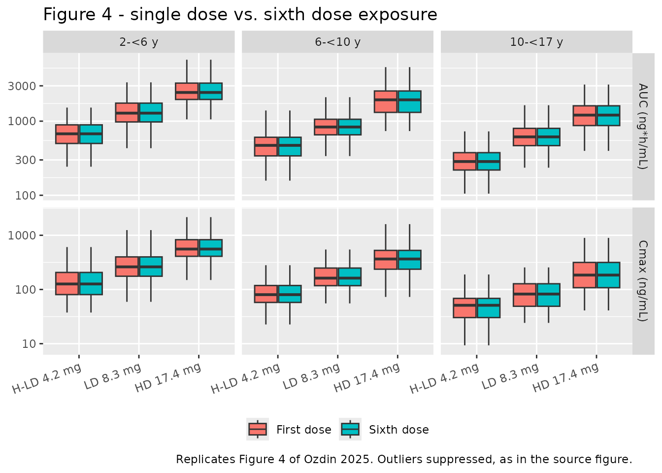
accum <- nca_long |>
  filter(PPTESTCD %in% c("cmax", "auclast")) |>
  select(id, agegrp, dosegrp, PPTESTCD, window, PPORRES) |>
  tidyr::pivot_wider(names_from = window, values_from = PPORRES) |>
  mutate(ratio = `Sixth dose` / `First dose`) |>
  group_by(PPTESTCD) |>
  summarise(`Median ratio` = median(ratio),
            `Min ratio` = min(ratio), `Max ratio` = max(ratio),
            .groups = "drop") |>
  rename("Parameter" = PPTESTCD)

knitr::kable(accum, digits = 5,
caption = "Accumulation ratio (sixth dose / first dose) across all 900 simulated subjects.")| Parameter | Median ratio | Min ratio | Max ratio |
|---|---|---|---|
| auclast | 1 | 1 | 1.00228 |
| cmax | 1 | 1 | 1.00225 |
# The paper's core claim: no accumulation with once-monthly dosing.
stopifnot(all(abs(accum$`Median ratio` - 1) < 0.01))
The accumulation ratio is 1.000 to within numerical precision, which the model’s parameters make inevitable: the terminal half-life is about 31 h (computed above), so a 720 h dosing interval is roughly 23 terminal half-lives and nothing carries over.
Between-subject-variability scale check
This is the quantitative version of point 2 in the source-trace
discussion. The cohort is re-solved under the alternative reading
omega^2 = CV^2 and the resulting exposure spread is
compared with what Ozdin 2025 Table 3 reports.
Cmax is the only metric with useful discriminating power: it is driven mostly by V1, where the two readings differ by 23% in variance (0.4054 versus 0.4998). AUC is driven by CL, where they differ by only 4% (0.1582 versus 0.1714), so AUC cannot separate them and is not shown.
Two refinements are needed to make the comparison interpretable at
100 subjects per arm. First, Table 3 reports the same
Cmax CV% for all three dose levels within an age band (63.9% throughout
the 2-to-under-6 band, 65.9% throughout 6-to-under-10, 71.0% throughout
10-to-under-17), confirming that the paper’s own simulated spread was
dose-independent; dose-normalised Cmax can therefore be pooled across
the three dose arms of a band, giving 300 subjects per estimate. Second,
the statistic compared is the standard deviation of log
Cmax rather than the raw-scale CV. A raw CV of a heavy-tailed
log-normal is a very noisy estimator at these sample sizes, whereas
sd(log(.)) is estimated with a Monte Carlo standard error
of about sd / sqrt(2(n - 1)), which is reported alongside
so the reader can judge whether a gap is meaningful. The published CV%
is put on the same scale via
omega = sqrt(log(1 + CV^2)).
dose_amt <- stats::setNames(dose_levels$amt, dose_levels$dose)

# sd(log(dose-normalised Cmax)) over the first monthly interval, pooled across
# the three dose arms of each age band, with its Monte Carlo standard error.
log_cmax_spread <- function(solved, reading) {
  solved |>
    filter(time <= tau) |>
    mutate(Cc = pmax(Cc, 0)) |>
    group_by(agegrp, dose, id) |>
    summarise(cmax = max(Cc), .groups = "drop") |>
    mutate(log_cmax_norm = log(cmax / dose_amt[as.character(dose)])) |>
    group_by(agegrp) |>
    summarise(`sd(log Cmax)` = sd(log_cmax_norm),
              `MC SE` = sd(log_cmax_norm) / sqrt(2 * (n() - 1)),
              n = n(), .groups = "drop") |>
    mutate(Reading = reading)
}

# The packaged model (exact-CV reading) reuses the simulation already run above.
spread_exact <- log_cmax_spread(
  sim |> select(id, time, Cc, agegrp, dose),
  "omega^2 = log(1 + CV^2)  [packaged]"
)

# The alternative reading: one extra solve on the identical event table.
mod_alt <- rxode2::ini(mod, etalcl = 0.414^2, etalvc = 0.707^2)
#> ℹ change initial estimate of `etalcl` to `0.171396`
#> ℹ change initial estimate of `etalvc` to `0.499849`
spread_alt <- rxode2::rxSolve(mod_alt, events, keep = c("agegrp", "dose"),
                              atol = 1e-12, rtol = 1e-10) |>
  as.data.frame() |>
  mutate(agegrp = factor(as.character(agegrp), levels = age_bands$agegrp),
         dose   = factor(as.character(dose),   levels = dose_levels$dose)) |>
  select(id, time, Cc, agegrp, dose) |>
  log_cmax_spread("omega^2 = CV^2  [rejected]")

# Table 3 CV% put on the sd(log) scale.
published_spread <- tibble::tibble(
  agegrp = factor(age_bands$agegrp, levels = age_bands$agegrp),
  cv = c(0.639, 0.659, 0.710),
  `sd(log Cmax)` = sqrt(log(1 + cv^2)),
  `MC SE` = NA_real_, n = NA_integer_,
  Reading = "Ozdin 2025 Table 3 (CV% -> sd log)"
) |>
  select(-cv)

omega_check <- bind_rows(published_spread, spread_exact, spread_alt) |>
  mutate(agegrp = factor(as.character(agegrp), levels = age_bands$agegrp)) |>
  arrange(agegrp) |>
  select(Reading, agegrp, `sd(log Cmax)`, `MC SE`, n)

omega_check |>
  rename("Age band" = agegrp, "N pooled" = n) |>
  knitr::kable(digits = 3,
caption = "Spread of log dose-normalised Cmax under the two readings of Table 2's BSV column, against the published value. Nominal omega_V1 is 0.637 under the packaged reading and 0.707 under the rejected one.")| Reading | Age band | sd(log Cmax) | MC SE | N pooled |
|---|---|---|---|---|
| Ozdin 2025 Table 3 (CV% -> sd log) | 2-<6 y | 0.585 | NA | NA |
| omega^2 = log(1 + CV^2) [packaged] | 2-<6 y | 0.606 | 0.025 | 300 |
| omega^2 = CV^2 [rejected] | 2-<6 y | 0.662 | 0.027 | 300 |
| Ozdin 2025 Table 3 (CV% -> sd log) | 6-<10 y | 0.601 | NA | NA |
| omega^2 = log(1 + CV^2) [packaged] | 6-<10 y | 0.598 | 0.024 | 300 |
| omega^2 = CV^2 [rejected] | 6-<10 y | 0.713 | 0.029 | 300 |
| Ozdin 2025 Table 3 (CV% -> sd log) | 10-<17 y | 0.639 | NA | NA |
| omega^2 = log(1 + CV^2) [packaged] | 10-<17 y | 0.664 | 0.027 | 300 |
| omega^2 = CV^2 [rejected] | 10-<17 y | 0.675 | 0.028 | 300 |
ref <- omega_check |> filter(grepl("^Ozdin", Reading))
omega_check |>
  filter(!grepl("^Ozdin", Reading)) |>
  group_by(Reading) |>
  summarise(
    `Mean deviation from published (sd log units)` =
      mean(`sd(log Cmax)` - ref$`sd(log Cmax)`[match(agegrp, ref$agegrp)]),
    `Mean abs deviation` =
      mean(abs(`sd(log Cmax)` - ref$`sd(log Cmax)`[match(agegrp, ref$agegrp)])),
    `Typical MC SE` = mean(`MC SE`),
    .groups = "drop"
  ) |>
  knitr::kable(digits = 3,
caption = "Agreement with the published Cmax spread, averaged over the three age bands. Smaller absolute deviation is better; compare it against the Monte Carlo standard error in the last column.")| Reading | Mean deviation from published (sd log units) | Mean abs deviation | Typical MC SE |
|---|---|---|---|
| omega^2 = CV^2 [rejected] | 0.075 | 0.075 | 0.028 |
| omega^2 = log(1 + CV^2) [packaged] | 0.014 | 0.016 | 0.025 |
How much this check proves. The packaged reading lands within one Monte Carlo standard error of the published spread in all three age bands (mean absolute deviation 0.016 against a Monte Carlo SE of about 0.026, and essentially no systematic bias). The rejected reading is high in every band, by about 0.075 on average, roughly three Monte Carlo standard errors. Per band the gap between the two readings ranges from about 0.4 to about 4 standard errors, so no single band is conclusive on its own, but the sign is the same in all three and the pooled discrepancy is well outside the noise.
This is nevertheless treated as corroborating rather than
decisive, because the comparison also depends on the assumed
weight distribution (see Assumptions), which contributes to the Cmax
spread independently of omega. The decisive evidence
remains the arithmetic agreement between
log(1 + 0.707^2) = 0.4054 and the control stream’s
$OMEGA starting value of 0.404706 – a 0.2% match where the
alternative would be 23% away – together with the
nlmixr2lib house convention.
Assumptions and deviations
- Weight distribution. Ozdin 2025 drew weights from CDC growth charts using a GAMLSS fit; that fitted object is not published. Weights here are truncated log-normal draws matched to the median and CV of each age band in Table 3. The 10-to-under-17 band is the one place this matters: the published distribution is slightly left-skewed (mean 50.3 kg below median 50.7 kg), which a log-normal cannot reproduce, so simulated Cmax in that band runs a few percent above the published median and its CV% a few points below.
-
Cohort size. 100 subjects per arm (900 total)
rather than the paper’s 1000 per age band, per the
nlmixr2libcap of 200 per arm. The comparison is against published medians, which are stable at this size. - Infusion duration. Fixed at 40 min for every arm, the phase 3 value (Methods section 2.1). The phase 1 infusions were about 10 min, which shifts Tmax but has almost no effect on AUC.
- Dose amounts. The nominal levels 4.2 / 8.3 / 17.4 mg from Methods section 2.6 are used for every subject. The actual per-subject encapsulated dose varied substantially (Table S2 reports CV 18-47% within dose level, and Table S4 shows observed low-dose amounts spanning 0.156-27.3 mg), because the mass loaded into the erythrocytes cannot be controlled exactly. Figure 4 of the paper labels the low and high doses 8.12 mg and 17.3 mg while Table 3 labels them 8.3 mg and 17.4 mg; the Table 3 values are used here for consistency with the exposures being compared.
-
Molecular-weight conversion. None is applied. Doses
are the mass of DSP encapsulated and concentrations are dexamethasone,
so a strictly mechanistic treatment would scale the dose by
FD = 0.76(516.4 / 392.464 g/mol). The paper introducesFDonly in the rejected semi-physiological model (supplement Figure S4 notes); the retained control stream doses the central compartment with the DSP amount directly, and reproducing Table 3 confirms that reading. ThecompartmentDataentries therefore describe amounts of dexamethasone on a DSP mass basis. -
DIS_HEALTHYorientation. The structural typicallclis shifted to the ataxia-telangiectasia patient state so thatDIS_HEALTHY = 1restores the paper’s printed healthy typical of 20.8 L/h. Simulating healthy adults requires settingDIS_HEALTHY = 1and supplying adult weights; every arm in this vignette is a patient arm. -
Residual error is not applied in the simulations.
All figures and tables show
Cc(the individual prediction), notsimwith residual error added. The phase 3 additive SD of 24.3 ng/mL is large relative to the tail concentrations, so adding it would dominate a semi-log profile plot; the published Table 3 and Table S3 exposures are likewise derived from model-predicted profiles (Methods section 2.6).
Errata and unreproducible source claims
-
The Discussion’s 20-30 day concentration is off by orders of magnitude. Ozdin 2025 Discussion states that “both LD and HD dose levels of eDSP show dexamethasone plasma concentrations of approximately 10^-3 ng/mL after 20-30 days (corresponding to 500-720 h) from dosing time”. With the Table 2 parameters the model predicts about 1e-6 ng/mL at 500 h and about 1e-7 ng/mL at 700 h for the low dose, three to four orders of magnitude lower. The arithmetic reason is that the beta-phase intercept is small: at the reference weight it is only about 0.3 ng/mL, not the roughly 90 ng/mL of Cmax, so the concentration is already far below 10^-3 ng/mL well before day 20. The paper’s own Figure 2 caption is consistent with the model rather than the Discussion, noting that 202 observations had IPRED below an LLOQ of 0.0005 ng/mL. The Discussion sentence appears to be an error, and the “sustained release for 20-30 days” narrative is a property of the observed data and of the rejected mechanistic release models, not of the retained two-compartment model, whose terminal half-life is about 31 h. The paper acknowledges this limitation directly: “the simplified two-compartment model does not explicitly capture the controlled, likely triphasic release from RBCs”.
sim |>
  filter(dose == "LD 8.3 mg", agegrp == "10-<17 y", dose_index == 1,
         t_after_dose %in% c(24, 240, 480, 720)) |>
  group_by(t_after_dose) |>
  summarise(`Median Cc (ng/mL)` = median(Cc), .groups = "drop") |>
  mutate(`Days after dose` = t_after_dose / 24, .before = 1) |>
  select(-t_after_dose) |>
  knitr::kable(digits = 10,
               caption = "Model-predicted low-dose tail concentrations, 10-<17 y. Compare with the Discussion's claim of approximately 1e-3 ng/mL at 500-720 h.")
Model-predicted low-dose tail concentrations, 10-<17 y. Compare with the Discussion’s claim of approximately 1e-3 ng/mL at 500-720 h. Days after dose Median Cc (ng/mL) 1 2.1046520625 10 0.0015474405 20 0.0000068471 Objective function values. Results section 3.2 quotes 2652.543 for the two-compartment model and 2724.38 for the three-compartment model, while the Table 2 note gives 8584.636 for the final model. The first pair evidently refers to the phase-1-only structural comparison and the third to the pooled final fit; the paper does not say so explicitly. No model parameter depends on this.
Adult counts in the abstract. The abstract describes the pooled population as “24 healthy adults and 109 AT patients”. Table 1 and Results section 3.1 make clear that the 24 are all adults (18 healthy from phase 1 plus 6 ataxia-telangiectasia patients from phase 3), not 24 healthy subjects. The model file uses the Table 1 reading: 18 subjects with
DIS_HEALTHY = 1and 115 withDIS_HEALTHY = 0.$THETAand$OMEGAin the supplement control stream are initial estimates, not final ones (CL 19.3324 vs. 20.8; V2 9.94667 vs. 16.8; PTNT 0.5 vs. 0.899). Every value in the model file comes from Table 2. The starting values are used only as corroborating evidence for the BSV scale, as described above.