Roscovitine (Leven 2020)
Source:vignettes/articles/Leven_2020_roscovitine.Rmd
Leven_2020_roscovitine.RmdModel and source
- Citation: Leven C, Schutz S, Audrezet MP, Nowak E, Meijer L, Montier T. Non-Linear Pharmacokinetics of Oral Roscovitine (Seliciclib) in Cystic Fibrosis Patients Chronically Infected with Pseudomonas aeruginosa: A Study on Population Pharmacokinetics with Monte Carlo Simulations. Pharmaceutics. 2020;12(11):1087. doi:10.3390/pharmaceutics12111087
- Description: Two-compartment parent-metabolite population PK model for oral roscovitine (seliciclib) and its carboxylate metabolite M3 in adults with cystic fibrosis chronically infected with Pseudomonas aeruginosa (Leven 2020), with a dose-dependent saturable first-pass effect (Emax-type fraction of the dose escaping first-pass conversion) and a sum-of-inverse-Gaussian-densities absorption input (two parallel roscovitine inputs, one pre-systemic M3 input sharing the first roscovitine input’s shape). The roscovitine and M3 central volumes share one apparent V/F, and roscovitine has no elimination route other than systemic conversion to M3.
- Article (open access): https://doi.org/10.3390/pharmaceutics12111087
Roscovitine (seliciclib) is an oral purine-analogue protein-kinase inhibitor investigated in cystic fibrosis (CF) for its effects on F508del-CFTR degradation and on alveolar-macrophage bactericidal activity. Leven 2020 characterised its pharmacokinetics and that of its main carboxylate metabolite M3 after the first oral dose in the ROSCO-CF phase IIa trial. The final model has three unusual features, all reproduced here:
-
A dose-dependent, saturable first-pass effect. The
fraction of the dose reaching the systemic circulation as roscovitine is
fdose = Dose / (Dose + D50)(Equation 7); the remainder,1 - fdose, enters the circulation as pre-formed M3. -
A sum-of-inverse-Gaussian absorption input without
any first-order absorption step (Equations 4-6): two parallel
roscovitine inputs weighted
pi1and1 - pi1, plus one M3 input whose shape is fixed to the first roscovitine input (TM3max = T1max,CVM3 = CV1, Section 3.2). -
No roscovitine elimination other than systemic conversion to
M3 (
kmet), and one apparent volumeV/Fshared by both molecules, because neither a parent elimination route nor a separate M3 volume was identifiable from oral data (Section 3.2).
The paper’s Appendix A prints the complete MLXTRAN structural model, which is what this implementation follows line by line.
Population
Twenty-three adults with CF (two CF-causing mutations including at least one F508del, FEV1 >= 40%, chronic Pseudomonas aeruginosa infection) received a single morning oral dose of 200 mg (n = 9), 400 mg (n = 7) or 800 mg (n = 7) roscovitine as 200 mg hard gelatin capsules, with PK sampled pre-dose and at 0.5, 1, 2, 4, 6, 8 and 12 h after the first dose (Sections 2.2-2.3). Median (range) age was 33 (22-51) years, weight 58 (48-90) kg, height 166 (158-182) cm and MDRD GFR 113 (61-202) mL/min; 10 were female and 15 took a proton-pump inhibitor (PPI; Table 2). The data comprised 138 roscovitine (19 BLQ) and 138 M3 (9 BLQ) concentrations (Table 1).
The same information is available programmatically via
readModelDb("Leven_2020_roscovitine")()$population.
Source trace
| Equation / parameter | Value | Source location |
|---|---|---|
led50 (D50) |
log(1190 umol) | Table 3 |
logitfrel (pi1) |
logit(0.285) | Table 3; logit-normal, Section 2.5 |
ltpeak_invgauss1 (T1max) |
log(0.676 h) | Table 3 |
e_conmed_ppi_tpeak_invgauss1 |
0.680 | Table 3, ‘beta (PPI = 1) on T1max’; Equation 9 |
ldtpeak_invgauss2 (dT2max) |
log(1.04 h) | Table 3; T2max = T1max + dT2max, Section 3.2 |
lcv_invgauss1, lcv_invgauss2 (CV1,
CV2) |
log(0.542), log(0.354) | Table 3 |
lvc (V/F) |
log(62.2 L) | Table 3 |
e_ht_vc |
6.47 | Table 3; Equation 10 with reference height 170 cm (Section 3.2) |
lk12, lk21
|
log(1.82), log(0.768) 1/h | Table 3 |
lkmet |
log(2.07 1/h) | Table 3 |
lkel_m3 (ke) |
log(2.58 1/h) | Table 3 |
| IIV variances | omega^2 of the Table 3 SDs | Table 3 (D50 0.689, T1max 0.452, dT2max 0.647, CV1 0.426, CV2 0.547, V/F 0.678, ke 0.393) |
| IIV covariances | corr x omega x omega | Table 3 (T1max-CV2 -0.839; dT2max-CV1 0.624) |
propSd |
0.297 | Table 3, ‘Roscovitine b1’ |
addSd_m3, propSd_m3
|
9.20 nmol/L, 0.271 | Table 3, ‘M3 a2’, ‘M3 b2’; combined error
sqrt(a^2 + b^2 f^2), Section 2.5 |
fdose = Dose / (Dose + D50) |
n/a | Equation 7; Appendix A Fr
|
MAT = Tmax / (sqrt(1 + 9/4 CV^4) - 3/2 CV^2) |
n/a | Equation 6; Appendix A MAT_1..MAT_3
|
inverse-Gaussian density IG(t)
|
n/a | Equation 5; Appendix A
inv_gauss_1..inv_gauss_3
|
d/dt(central), d/dt(peripheral1),
d/dt(central_m3)
|
n/a | Figure 2; Appendix A dArosco, dAroscop,
dAM3
|
Cc = central / vc * 1000,
Cc_m3 = central_m3 / vc * 1000
|
n/a | Appendix A C_rosco, C_M3 (nmol/L) |
Implementation notes
-
Dose units. The model is dosed in
micromoles of roscovitine and predicts both analytes in
nmol/L, exactly as the paper fitted it (Section 2.3:
doses converted to umol, concentrations to nmol/L, molecular weights
354.45 g/mol for roscovitine and 368.43 g/mol for M3). D50 is therefore
in umol: a 200 mg dose is
200 / 354.45 * 1000 = 564.3umol. -
The input function. Monolix evaluates the
inverse-Gaussian inputs from the dose amount (
amtDose) and the time since dosing. rxode2 exposes the same two quantities aspodo(depot)andtad(depot). The dose is placed indepot, which is emptied at exactly the prescribed input rate, so the total amount in the system is conserved; the mass-balance check below confirms that each dose is delivered once and completely. -
Repeated dosing. The model was fitted to the first
dose only. With
podo()/tad()a new dose restarts the input clock, which is accurate as long as the previous dose has been absorbed (the slower density has a mean absorption time of about 2 h at typical values, so this holds for the once-daily ROSCO-CF regimen).
Molecular weights and dose conversion
MW_ROSCO <- 354.45 # g/mol, Section 2.3
MW_M3 <- 368.43 # g/mol, Section 2.3
mg_to_umol <- function(mg) mg / MW_ROSCO * 1000

mod <- rxode2::rxode2(readModelDb("Leven_2020_roscovitine"))
#> ℹ parameter labels from comments will be replaced by 'label()'
# The explicit ODEs must be kept: a model with a volume and micro-constants
# must not be silently converted to a closed-form linear compartment model.
stopifnot(is.null(mod$linCmt))
ini_vals <- mod$theta
Event-table builder
# Event tables are data frames, so the covariate columns survive. The model
# declares two endpoints, so observation rows sit on a real ODE state
# (cmt = "central") and nominate an endpoint with dvid = 1; both observables,
# Cc and Cc_m3, come back as columns on every observation row.
build_events <- function(cohort, obs_times) {
  dose <- cohort |>
    dplyr::transmute(id, time = 0, amt = mg_to_umol(dose_mg), evid = 1L,
                     cmt = "depot", dvid = NA_integer_, HT, CONMED_PPI)
  obs <- cohort |>
    dplyr::select(id, HT, CONMED_PPI) |>
    tidyr::crossing(time = obs_times) |>
    dplyr::mutate(amt = 0, evid = 0L, cmt = "central", dvid = 1L) |>
    dplyr::select(id, time, amt, evid, cmt, dvid, HT, CONMED_PPI)
  dplyr::bind_rows(dose, obs) |>
    dplyr::arrange(id, time, dplyr::desc(evid))
}
Deterministic checks
First-pass fraction
The Results (Section 3.2) state that D50 = 1190 umol gives
Fr = 0.32, 0.49 and 0.65 at 200, 400 and 800 mg. The
model’s own fdose at the dose time is compared against
those printed values; the tolerance is half of the last printed
digit.
typ <- rxode2::zeroRe(mod)
doses_mg <- c(200, 400, 800)
typ_cohort <- tibble::tibble(id = 1:3, dose_mg = doses_mg, HT = 170, CONMED_PPI = 0)
typ_times <- c(0, exp(seq(log(0.001), log(0.05), length.out = 40)), seq(0.1, 96, by = 0.05))
typ_sim <- rxode2::rxSolve(typ, build_events(typ_cohort, typ_times),
                           returnType = "data.frame", atol = 1e-12, rtol = 1e-10,
                           maxsteps = 1e6) |>
  dplyr::left_join(typ_cohort, by = "id")
#> ℹ omega/sigma items treated as zero: 'etaled50', 'etaltpeak_invgauss1', 'etalcv_invgauss2', 'etaldtpeak_invgauss2', 'etalcv_invgauss1', 'etalvc', 'etalkel_m3'
#> Warning: multi-subject simulation without without 'omega'

fdose_tab <- typ_sim |>
  dplyr::group_by(dose_mg) |>
  dplyr::summarise(fdose = dplyr::last(fdose), .groups = "drop") |>
  dplyr::mutate(published = c(0.32, 0.49, 0.65))
knitr::kable(fdose_tab |> dplyr::rename("Dose (mg)" = dose_mg, "Model fdose" = fdose,
                                        "Published Fr" = published),
digits = 4, caption = "Fraction of the dose escaping first-pass conversion.")| Dose (mg) | Model fdose | Published Fr |
|---|---|---|
| 200 | 0.3216 | 0.32 |
| 400 | 0.4867 | 0.49 |
| 800 | 0.6548 | 0.65 |
Mass balance
Roscovitine leaves the body only by conversion to M3, and M3 only by
ke. Therefore, for any subject, the whole dose must be
eliminated as M3 and the fraction fdose must pass through
systemic roscovitine:
-
ke * V * AUC0-inf(M3) / 1000 = Dose(umol), -
kmet * V * AUC0-inf(roscovitine) / 1000 = fdose * Dose.
Both sides come from the same solve, so the only discrepancy allowed is numerical integration and trapezoidal error. An input function that delivered nothing, delivered a dose twice, or put the pre-systemic fraction in the wrong compartment would fail these by tens of percent.
trap <- function(x, y) sum(diff(x) * (head(y, -1) + tail(y, -1)) / 2)
mb <- typ_sim |>
  dplyr::group_by(dose_mg) |>
  dplyr::summarise(
    dose_umol = mg_to_umol(dplyr::first(dose_mg)),
    fdose = dplyr::last(fdose),
    auc_m3 = trap(time, Cc_m3),
    auc_rosco = trap(time, Cc),
    depot_end = dplyr::last(depot),
    vc = dplyr::last(vc), kel_m3 = dplyr::last(kel_m3), kmet = dplyr::last(kmet),
    .groups = "drop"
  ) |>
  dplyr::mutate(
    m3_recovered = kel_m3 * vc * auc_m3 / 1000 / dose_umol,
    rosco_recovered = kmet * vc * auc_rosco / 1000 / (fdose * dose_umol)
  )
knitr::kable(mb |> dplyr::select(dose_mg, m3_recovered, rosco_recovered, depot_end) |>
               dplyr::rename("Dose (mg)" = dose_mg,
                             "M3 eliminated / dose" = m3_recovered,
                             "Systemic roscovitine / (fdose x dose)" = rosco_recovered,
                             "Depot at 96 h (umol)" = depot_end),
digits = 6, caption = "Typical-value mass balance (reference height 170 cm, no PPI).")| Dose (mg) | M3 eliminated / dose | Systemic roscovitine / (fdose x dose) | Depot at 96 h (umol) |
|---|---|---|---|
| 200 | 1 | 1 | 0 |
| 400 | 1 | 1 | 0 |
| 800 | 1 | 1 | 0 |
Virtual cohort
The paper’s Monte Carlo simulations used 1000 patients per scenario
but do not state the covariate values. Simulating at the
reference height of 170 cm, with PPI use drawn at the
observed prevalence (15 of 23), is consistent with the published medians
(tables below), whereas a cohort whose heights span the observed 158-182
cm range is expected to give higher roscovitine and M3 exposure because
V/F scales as (HT / 170)^6.47 and the observed median
height (166 cm) lies below the reference (see the sensitivity section at
the end). The primary cohort therefore uses 170 cm; each dose arm has
200 virtual patients.
rxode2::rxSetSeed(2020)
set.seed(2020)
n_per_arm <- 200

# Heights for the sensitivity cohort: normal around the observed median, redrawn
# (never clamped) until inside the observed 158-182 cm range (Table 2).
draw_height <- function(n) {
  out <- numeric(0)
  while (length(out) < n) {
    x <- rnorm(n, 166, 7)
    out <- c(out, x[x >= 158 & x <= 182])
  }
  out[seq_len(n)]
}

make_cohort <- function(n, dose_mg, ppi = NULL, height = NULL, id_offset = 0L) {
  tibble::tibble(
    id = id_offset + seq_len(n),
    dose_mg = dose_mg,
    HT = if (is.null(height)) 170 else height(n),
    CONMED_PPI = if (is.null(ppi)) rbinom(n, 1, 15 / 23) else ppi
  )
}

dose_cohort <- dplyr::bind_rows(
  make_cohort(n_per_arm, 200, id_offset = 0L),
  make_cohort(n_per_arm, 400, id_offset = 1000L),
  make_cohort(n_per_arm, 800, id_offset = 2000L)
) |>
  dplyr::mutate(treatment = paste(dose_mg, "mg"))

obs_times <- sort(unique(c(seq(0, 12, by = 0.1))))
dose_sim <- rxode2::rxSolve(mod, build_events(dose_cohort, obs_times),
                            returnType = "data.frame") |>
  dplyr::left_join(dose_cohort |> dplyr::select(id, dose_mg, treatment), by = "id")
Simulated profiles by dose (replicates Figure 7)
band <- dose_sim |>
  dplyr::select(treatment, time, Roscovitine = Cc, `M3 metabolite` = Cc_m3) |>
  tidyr::pivot_longer(c(Roscovitine, `M3 metabolite`), names_to = "analyte", values_to = "conc") |>
  dplyr::group_by(treatment, analyte, time) |>
  dplyr::summarise(p10 = quantile(conc, 0.1), p50 = median(conc), p90 = quantile(conc, 0.9),
                   .groups = "drop") |>
  dplyr::mutate(analyte = factor(analyte, c("Roscovitine", "M3 metabolite")),
                treatment = factor(treatment, c("200 mg", "400 mg", "800 mg")))

ggplot(band, aes(time, p50)) +
  geom_ribbon(aes(ymin = p10, ymax = p90), fill = "steelblue", alpha = 0.3) +
  geom_line(colour = "steelblue4") +
  facet_grid(analyte ~ treatment, scales = "free_y") +
  labs(x = "Time (h)", y = "Concentration (nmol/L)",
       caption = "Median and 10th-90th percentiles; replicates Figure 7 of Leven 2020.")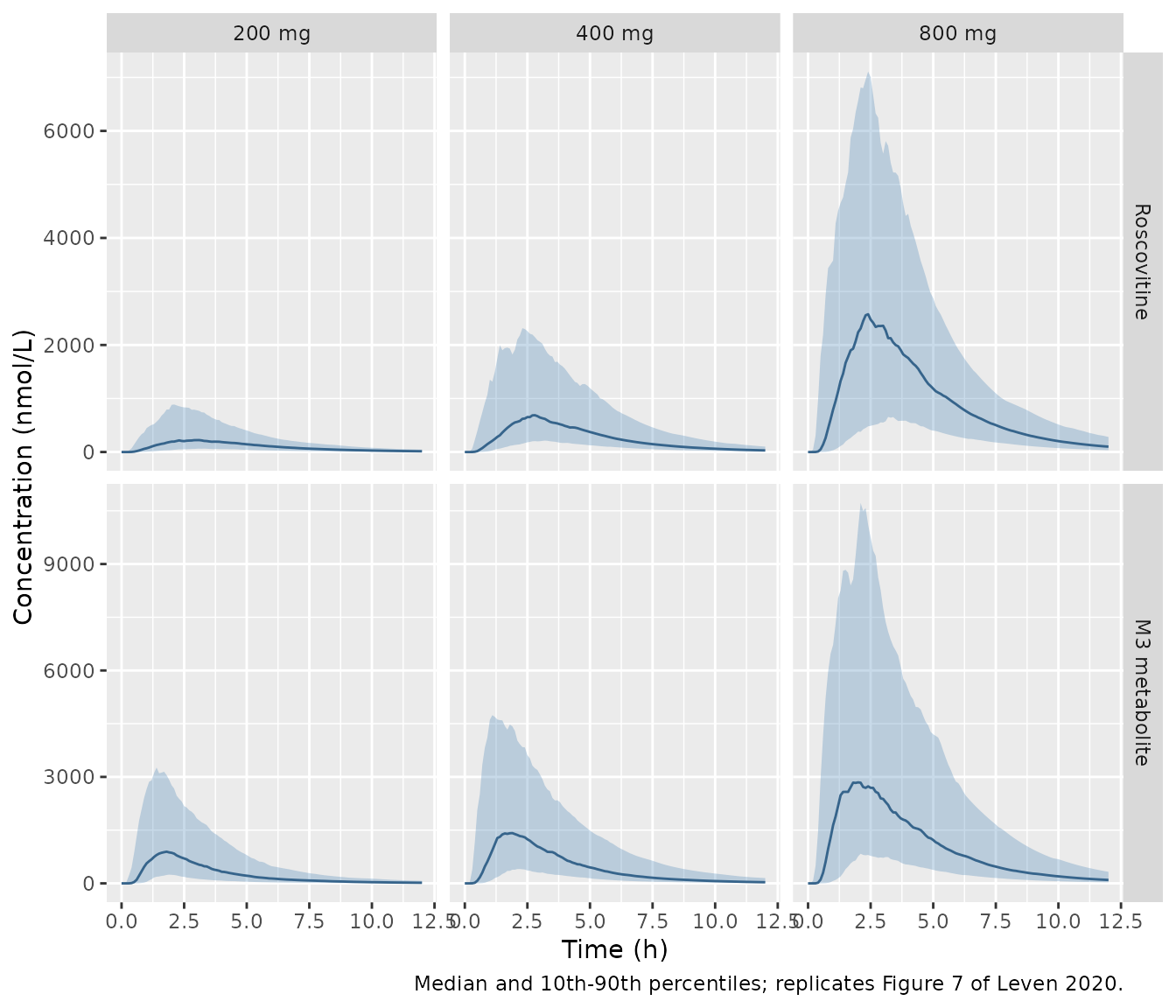
As in Figure 7, roscovitine exposure rises more than proportionally with dose while the M3 peak, which precedes the roscovitine peak because its input shares the faster first density, rises less than proportionally. Over an infinite horizon M3 exposure is exactly dose-proportional (every umol of roscovitine is eventually eliminated as M3, as the mass-balance check shows); the less-than-proportional AUC0-12h arises because at higher doses a larger share of the dose passes through systemic roscovitine and its peripheral compartment before becoming M3, so more of the M3 is formed after 12 h. Both statements are asserted below the PKNCA table.
PKNCA: AUC0-12h by dose (Section 3.3)
The paper reports the median (interquartile range) simulated AUC0-12h in ng.h/mL. The model concentrations are converted from nmol/L to ng/mL with the molecular weights above.
# The inverse-Gaussian input is vanishingly small just after the dose, and the
# integrator can return values a few ulps below zero there (of order 1e-17
# nmol/L). PKNCA returns NA for an AUC over a negative concentration, so the
# undershoot is first asserted to be pure numerical noise -- relative to each
# subject's peak -- and then floored at zero.
nca_input <- function(sim, conc_col, mw) {
  out <- sim |>
    dplyr::filter(!is.na(.data[[conc_col]])) |>
    dplyr::transmute(treatment, id, time, Cc = .data[[conc_col]] * mw / 1000) |>
    dplyr::group_by(id) |>
    dplyr::mutate(peak = max(Cc)) |>
    dplyr::ungroup()
  stopifnot(all(out$Cc >= -1e-9 * out$peak))
  out |>
    dplyr::mutate(Cc = pmax(Cc, 0)) |>
    dplyr::select(-peak)
}
run_nca <- function(conc_df, cohort) {
  conc_obj <- PKNCA::PKNCAconc(conc_df, Cc ~ time | treatment + id,
                               concu = "ng/mL", timeu = "h")
  dose_obj <- PKNCA::PKNCAdose(
    cohort |> dplyr::transmute(treatment, id, time = 0, dose = dose_mg),
    dose ~ time | treatment + id, doseu = "mg"
  )
  intervals <- data.frame(start = 0, end = 12, auclast = TRUE, cmax = TRUE, tmax = TRUE)
  PKNCA::pk.nca(PKNCA::PKNCAdata(conc_obj, dose_obj, intervals = intervals))
}
nca_rosco <- run_nca(nca_input(dose_sim, "Cc", MW_ROSCO), dose_cohort)
nca_m3 <- run_nca(nca_input(dose_sim, "Cc_m3", MW_M3), dose_cohort)

published_rosco <- tibble::tribble(
  ~treatment, ~auclast,
  "200 mg", 477,
  "400 mg", 1436,
  "800 mg", 3711
)
published_m3 <- tibble::tribble(
  ~treatment, ~auclast,
  "200 mg", 1293,
  "400 mg", 2557,
  "800 mg", 4888
)
cmp <- dplyr::bind_rows(
  nlmixr2lib::ncaComparisonTable(nca_rosco, published_rosco, by = "treatment",
                                 params = "auclast", units = c(auclast = "ng*h/mL"),
                                 tolerance_pct = 20) |>
    dplyr::mutate(analyte = "Roscovitine"),
  nlmixr2lib::ncaComparisonTable(nca_m3, published_m3, by = "treatment",
                                 params = "auclast", units = c(auclast = "ng*h/mL"),
                                 tolerance_pct = 20) |>
    dplyr::mutate(analyte = "M3")
)
cmp |>
  dplyr::relocate(analyte) |>
  dplyr::rename("Analyte" = analyte, "Dose" = treatment) |>
  knitr::kable(caption = paste(
    "Simulated median AUC0-12h versus the Monte Carlo medians of Leven 2020",
    "Section 3.3. * differs by more than 20%."
))| Analyte | NCA parameter | Dose | Reference | Simulated | % diff |
|---|---|---|---|---|---|
| Roscovitine | AUClast (ng*h/mL) | 200 mg | 477 | 439 | -8.0% |
| Roscovitine | AUClast (ng*h/mL) | 400 mg | 1440 | 1240 | -13.8% |
| Roscovitine | AUClast (ng*h/mL) | 800 mg | 3710 | 4210 | +13.4% |
| M3 | AUClast (ng*h/mL) | 200 mg | 1290 | 1250 | -3.1% |
| M3 | AUClast (ng*h/mL) | 400 mg | 2560 | 2290 | -10.3% |
| M3 | AUClast (ng*h/mL) | 800 mg | 4890 | 4820 | -1.4% |
auc_tab <- function(nca, analyte) {
  as.data.frame(nca$result) |>
    dplyr::filter(PPTESTCD == "auclast") |>
    dplyr::select(treatment, id, auc = PPORRES) |>
    dplyr::mutate(analyte = analyte)
}
auc_all <- dplyr::bind_rows(auc_tab(nca_rosco, "rosco"), auc_tab(nca_m3, "m3"))
iqr_sim <- auc_all |>
  dplyr::group_by(analyte, treatment) |>
  dplyr::summarise(q25 = quantile(auc, 0.25), median = median(auc), q75 = quantile(auc, 0.75),
                   .groups = "drop")
iqr_pub <- tibble::tribble(
  ~analyte, ~treatment, ~pub_q25, ~pub_median, ~pub_q75,
  "rosco", "200 mg", 259, 477, 847,
  "rosco", "400 mg", 850, 1436, 2327,
  "rosco", "800 mg", 2335, 3711, 6329,
  "m3", "200 mg", 753, 1293, 2198,
  "m3", "400 mg", 1556, 2557, 4294,
  "m3", "800 mg", 2893, 4888, 8559
)
iqr_cmp <- dplyr::inner_join(iqr_sim, iqr_pub, by = c("analyte", "treatment"))
knitr::kable(iqr_cmp |>
               dplyr::rename("Analyte" = analyte, "Dose" = treatment,
                             "Sim. Q1" = q25, "Sim. median" = median, "Sim. Q3" = q75,
                             "Pub. Q1" = pub_q25, "Pub. median" = pub_median, "Pub. Q3" = pub_q75),
             digits = 0,
caption = "Simulated versus published AUC0-12h quartiles (ng.h/mL).")| Analyte | Dose | Sim. Q1 | Sim. median | Sim. Q3 | Pub. Q1 | Pub. median | Pub. Q3 |
|---|---|---|---|---|---|---|---|
| m3 | 200 mg | 724 | 1253 | 2016 | 753 | 1293 | 2198 |
| m3 | 400 mg | 1491 | 2293 | 3563 | 1556 | 2557 | 4294 |
| m3 | 800 mg | 3154 | 4821 | 8914 | 2893 | 4888 | 8559 |
| rosco | 200 mg | 255 | 439 | 807 | 259 | 477 | 847 |
| rosco | 400 mg | 765 | 1237 | 2046 | 850 | 1436 | 2327 |
| rosco | 800 mg | 2808 | 4207 | 6495 | 2335 | 3711 | 6329 |
# Assert on the centre and on robust quantiles only. A 200-per-arm median of
# this highly variable absorption has a sampling error of several percent per
# arm, so the tight check is on the pooled centre across the six analyte-dose
# rows, and the per-row check only has to catch gross errors. A mis-transcribed
# volume, D50 or rate constant moves every row by tens of percent.
lr <- function(sim, pub) log(sim / pub)
stopifnot(
  abs(median(lr(iqr_cmp$median, iqr_cmp$pub_median))) < log(1.1),
  all(abs(lr(iqr_cmp$median, iqr_cmp$pub_median)) < log(1.3)),
  abs(median(lr(iqr_cmp$q25, iqr_cmp$pub_q25))) < log(1.15),
  abs(median(lr(iqr_cmp$q75, iqr_cmp$pub_q75))) < log(1.15)
)

# Dose proportionality (Figure 7 narrative): a fourfold dose increase raises
# the median roscovitine AUC0-12h well over fourfold (7.8-fold in the paper)
# and the median M3 AUC0-12h by less than the paper's 3.8-fold plus margin.
med <- function(a, d) iqr_sim$median[iqr_sim$analyte == a & iqr_sim$treatment == d]
stopifnot(
  med("rosco", "800 mg") / med("rosco", "200 mg") > 5,
  med("m3", "800 mg") / med("m3", "200 mg") < 4.5
)

# The M3 peak precedes the roscovitine peak in every dose arm.
tmax_med <- dplyr::bind_rows(
  as.data.frame(nca_rosco$result) |> dplyr::mutate(analyte = "rosco"),
  as.data.frame(nca_m3$result) |> dplyr::mutate(analyte = "m3")
) |>
  dplyr::filter(PPTESTCD == "tmax") |>
  dplyr::group_by(analyte, treatment) |>
  dplyr::summarise(tmax = median(PPORRES), .groups = "drop") |>
  tidyr::pivot_wider(names_from = analyte, values_from = tmax)
knitr::kable(tmax_med |> dplyr::rename("Dose" = treatment, "Median Tmax M3 (h)" = m3,
                                       "Median Tmax roscovitine (h)" = rosco),
digits = 2)| Dose | Median Tmax M3 (h) | Median Tmax roscovitine (h) |
|---|---|---|
| 200 mg | 1.65 | 2.6 |
| 400 mg | 1.80 | 2.5 |
| 800 mg | 2.00 | 2.5 |
AUC ratio by dose (replicates Figure 8)
ratio <- auc_all |>
  tidyr::pivot_wider(names_from = analyte, values_from = auc) |>
  dplyr::mutate(ratio = rosco / m3 * MW_M3 / MW_ROSCO)
The ratio above is computed on molar AUCs (the ng.h/mL values
multiplied back by MW_M3 / MW_ROSCO), matching the paper’s
nmol/L modelling scale.
ggplot(ratio, aes(treatment, ratio, fill = treatment)) +
  geom_violin(alpha = 0.6) +
  geom_boxplot(width = 0.15, outlier.size = 0.5, fill = "white") +
  labs(x = "Roscovitine dose", y = "Roscovitine / M3 AUC ratio", fill = "Dose",
       caption = "Replicates Figure 8 of Leven 2020.")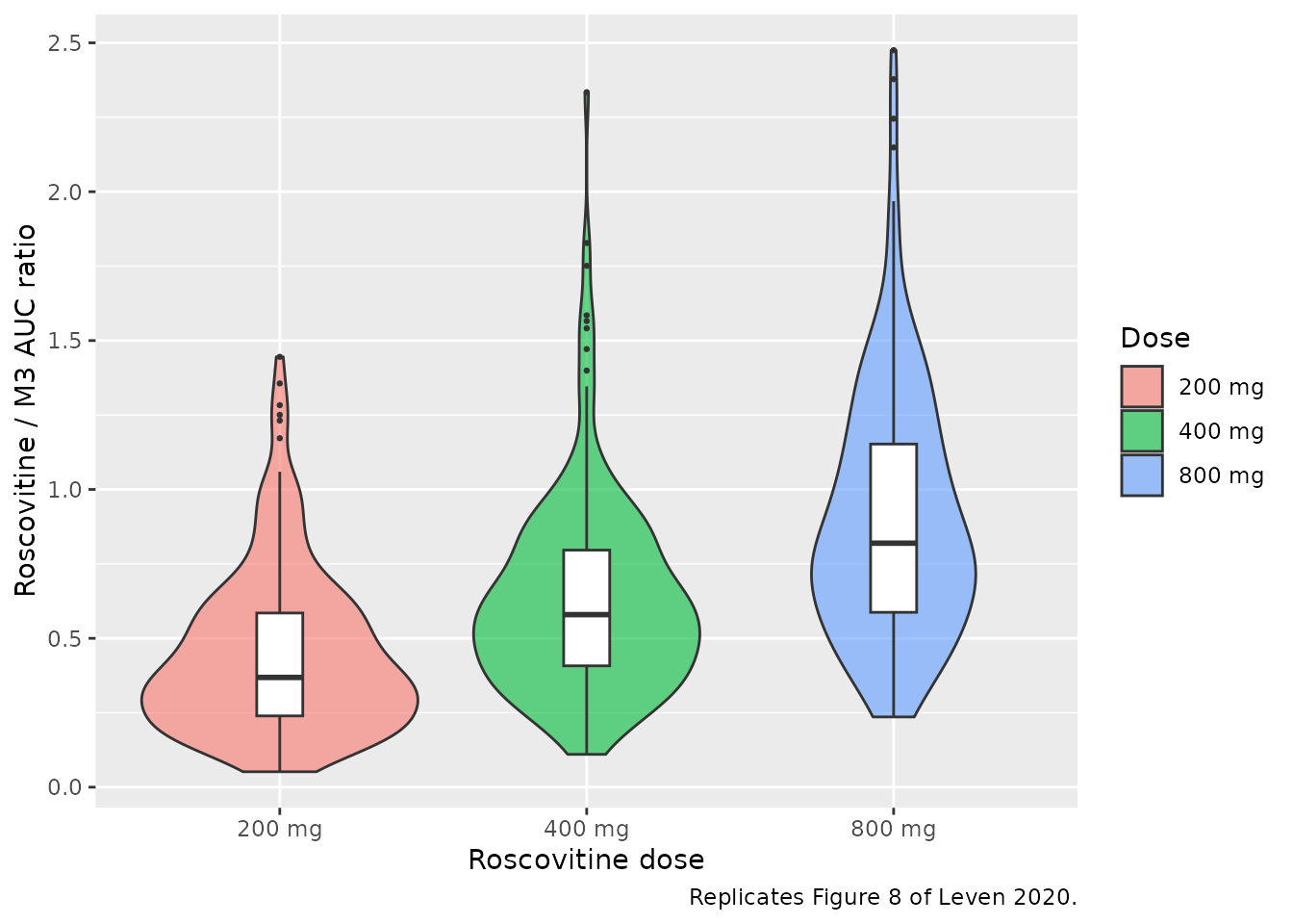
ratio_med <- ratio |>
  dplyr::group_by(treatment) |>
  dplyr::summarise(median_ratio = median(ratio), .groups = "drop")
knitr::kable(ratio_med |> dplyr::rename("Dose" = treatment, "Median AUC ratio" = median_ratio),
digits = 2)| Dose | Median AUC ratio |
|---|---|
| 200 mg | 0.37 |
| 400 mg | 0.58 |
| 800 mg | 0.82 |
The paper reports the median roscovitine/M3 AUC ratio rising from 0.37 at 200 mg to 0.79 at 800 mg (Section 3.3).
r200 <- ratio_med$median_ratio[ratio_med$treatment == "200 mg"]
r800 <- ratio_med$median_ratio[ratio_med$treatment == "800 mg"]
stopifnot(abs(r200 / 0.37 - 1) < 0.2, abs(r800 / 0.79 - 1) < 0.2)
The ratio’s median is taken on molar AUCs because the paper’s own model works in nmol/L; on ng.h/mL the ratio is smaller by the factor 354.45 / 368.43 (about 4%), which is within the tolerance either way.
Effect of proton-pump inhibitors at 400 mg (replicates Figures 9 and 10)
ppi_cohort <- dplyr::bind_rows(
  make_cohort(n_per_arm, 400, ppi = 0L, id_offset = 5000L),
  make_cohort(n_per_arm, 400, ppi = 1L, id_offset = 6000L)
) |>
  dplyr::mutate(treatment = paste0("400 mg, PPI = ", CONMED_PPI))
ppi_sim <- rxode2::rxSolve(mod, build_events(ppi_cohort, obs_times),
                           returnType = "data.frame") |>
  dplyr::left_join(ppi_cohort |> dplyr::select(id, dose_mg, treatment), by = "id")

ppi_band <- ppi_sim |>
  dplyr::select(treatment, time, Roscovitine = Cc, `M3 metabolite` = Cc_m3) |>
  tidyr::pivot_longer(c(Roscovitine, `M3 metabolite`), names_to = "analyte", values_to = "conc") |>
  dplyr::group_by(treatment, analyte, time) |>
  dplyr::summarise(p10 = quantile(conc, 0.1), p50 = median(conc), p90 = quantile(conc, 0.9),
                   .groups = "drop") |>
  dplyr::mutate(analyte = factor(analyte, c("Roscovitine", "M3 metabolite")))

ggplot(ppi_band, aes(time, p50)) +
  geom_ribbon(aes(ymin = p10, ymax = p90), fill = "steelblue", alpha = 0.3) +
  geom_line(colour = "steelblue4") +
  facet_grid(analyte ~ treatment, scales = "free_y") +
  labs(x = "Time (h)", y = "Concentration (nmol/L)",
       caption = "Median and 10th-90th percentiles; replicates Figure 9 of Leven 2020.")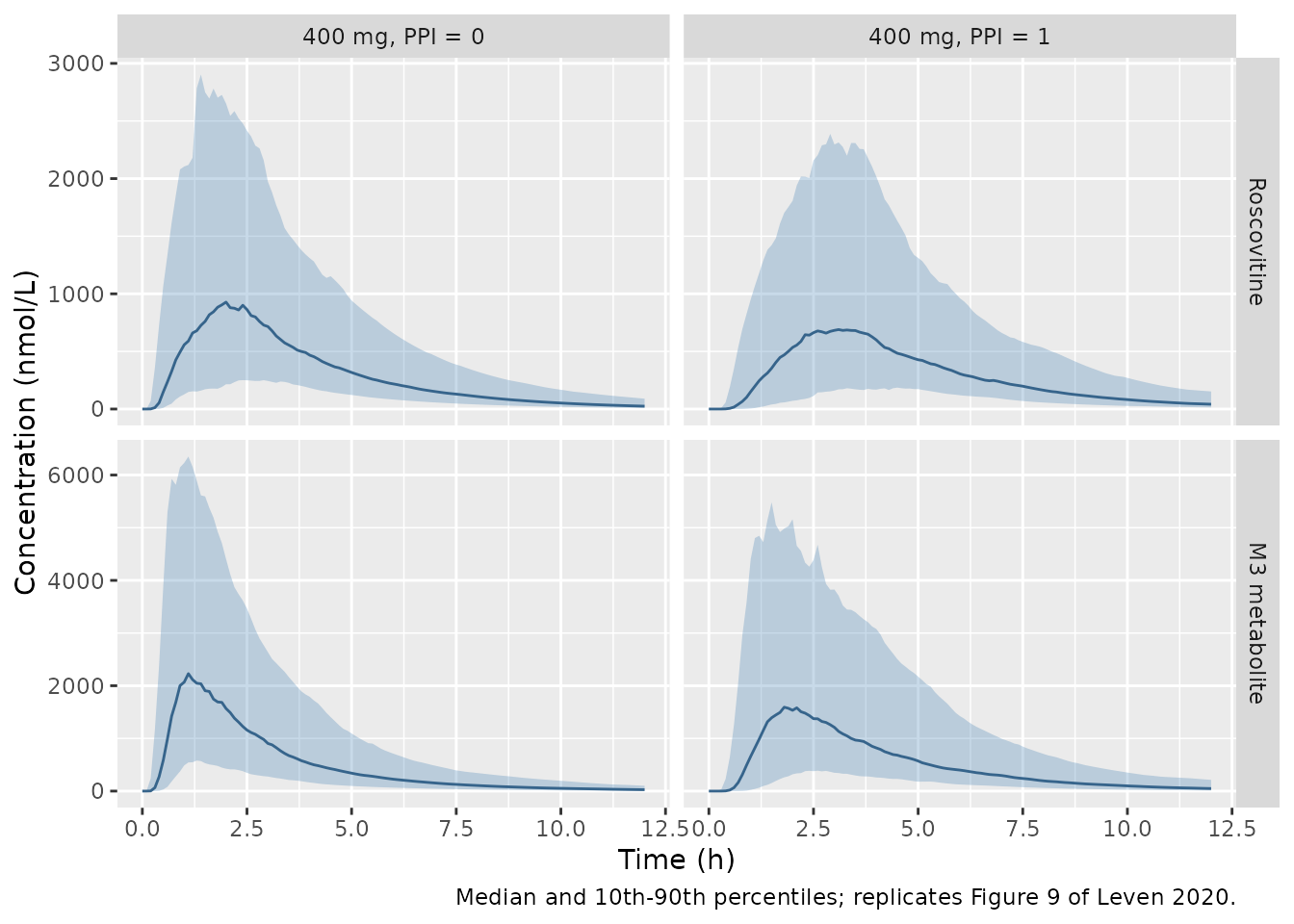
nca_ppi_rosco <- run_nca(nca_input(ppi_sim, "Cc", MW_ROSCO), ppi_cohort)
nca_ppi_m3 <- run_nca(nca_input(ppi_sim, "Cc_m3", MW_M3), ppi_cohort)
ppi_res <- dplyr::bind_rows(
  as.data.frame(nca_ppi_rosco$result) |> dplyr::mutate(analyte = "rosco"),
  as.data.frame(nca_ppi_m3$result) |> dplyr::mutate(analyte = "m3")
) |>
  dplyr::filter(PPTESTCD %in% c("auclast", "tmax")) |>
  dplyr::select(analyte, treatment, id, PPTESTCD, PPORRES) |>
  tidyr::pivot_wider(names_from = PPTESTCD, values_from = PPORRES)
ppi_sum <- ppi_res |>
  dplyr::group_by(analyte, treatment) |>
  dplyr::summarise(median_tmax = median(tmax), median_auc = median(auclast), .groups = "drop")
knitr::kable(ppi_sum |> dplyr::rename("Analyte" = analyte, "Group" = treatment,
                                      "Median Tmax (h)" = median_tmax,
                                      "Median AUC0-12h (ng.h/mL)" = median_auc),
digits = 2)| Analyte | Group | Median Tmax (h) | Median AUC0-12h (ng.h/mL) |
|---|---|---|---|
| m3 | 400 mg, PPI = 0 | 1.2 | 2418.80 |
| m3 | 400 mg, PPI = 1 | 2.1 | 2707.87 |
| rosco | 400 mg, PPI = 0 | 2.0 | 1452.77 |
| rosco | 400 mg, PPI = 1 | 2.7 | 1473.20 |
ppi_ratio <- ppi_res |>
  dplyr::select(analyte, treatment, id, auclast) |>
  tidyr::pivot_wider(names_from = analyte, values_from = auclast) |>
  dplyr::mutate(ratio = rosco / m3 * MW_M3 / MW_ROSCO)
ggplot(ppi_ratio, aes(treatment, ratio, fill = treatment)) +
  geom_violin(alpha = 0.6) +
  geom_boxplot(width = 0.15, outlier.size = 0.5, fill = "white") +
  labs(x = NULL, y = "Roscovitine / M3 AUC ratio", fill = NULL,
       caption = "Replicates Figure 10 of Leven 2020.")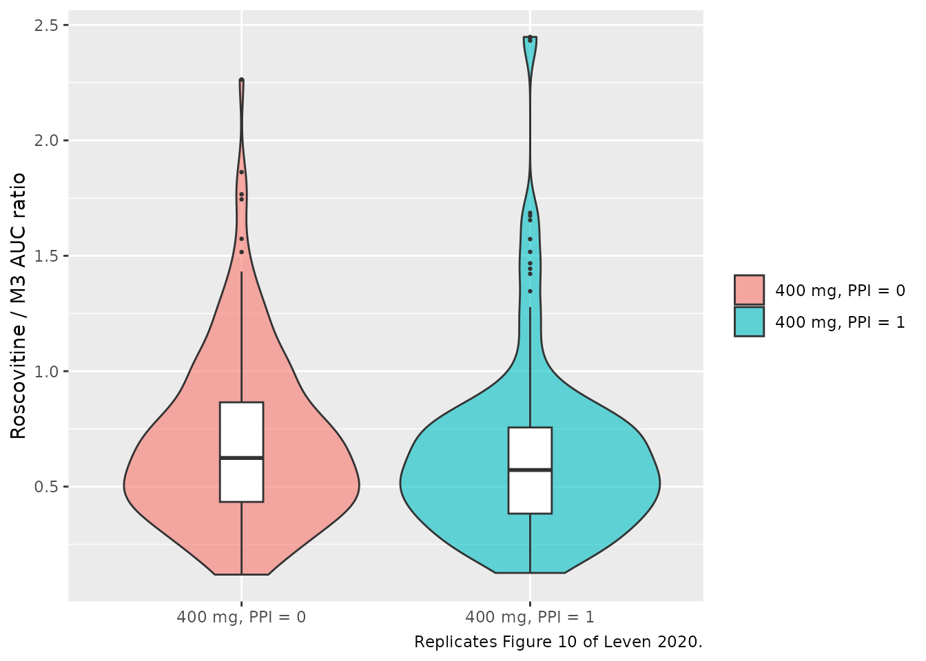
PPI use nearly doubles T1max (exp(0.680) = 1.97), which
delays both the roscovitine peak and – because the pre-systemic M3 input
shares T1max – the M3 peak, and flattens both, while leaving exposure
essentially unchanged (Figures 9 and 10: “no obvious effect on plasma
exposure or AUCrosco/AUCM3 ratios”).
tm <- function(a, g) ppi_sum$median_tmax[ppi_sum$analyte == a & ppi_sum$treatment == g]
au <- function(a, g) ppi_sum$median_auc[ppi_sum$analyte == a & ppi_sum$treatment == g]
ratio_by_ppi <- ppi_ratio |>
  dplyr::group_by(treatment) |>
  dplyr::summarise(m = median(ratio), .groups = "drop")
stopifnot(
  # Both peaks move later by a clear margin (about 1 h at typical values).
  tm("rosco", "400 mg, PPI = 1") - tm("rosco", "400 mg, PPI = 0") > 0.4,
  tm("m3", "400 mg, PPI = 1") - tm("m3", "400 mg, PPI = 0") > 0.4,
  # Exposure is essentially unchanged: magnitude, not sign.
  abs(log(au("rosco", "400 mg, PPI = 1") / au("rosco", "400 mg, PPI = 0"))) < log(1.3),
  abs(log(au("m3", "400 mg, PPI = 1") / au("m3", "400 mg, PPI = 0"))) < log(1.3),
  abs(log(ratio_by_ppi$m[2] / ratio_by_ppi$m[1])) < log(1.3)
)
Sensitivity: cohort with the observed height range
ht_cohort <- dplyr::bind_rows(
  make_cohort(n_per_arm, 200, height = draw_height, id_offset = 7000L),
  make_cohort(n_per_arm, 400, height = draw_height, id_offset = 8000L),
  make_cohort(n_per_arm, 800, height = draw_height, id_offset = 9000L)
) |>
  dplyr::mutate(treatment = paste(dose_mg, "mg"))
ht_sim <- rxode2::rxSolve(mod, build_events(ht_cohort, obs_times),
                          returnType = "data.frame") |>
  dplyr::left_join(ht_cohort |> dplyr::select(id, dose_mg, treatment), by = "id")
ht_auc <- dplyr::bind_rows(
  auc_tab(run_nca(nca_input(ht_sim, "Cc", MW_ROSCO), ht_cohort), "rosco"),
  auc_tab(run_nca(nca_input(ht_sim, "Cc_m3", MW_M3), ht_cohort), "m3")
) |>
  dplyr::group_by(analyte, treatment) |>
  dplyr::summarise(median_observed_heights = median(auc), .groups = "drop")
ht_cmp <- iqr_cmp |>
  dplyr::select(analyte, treatment, median_170 = median, pub_median) |>
  dplyr::inner_join(ht_auc, by = c("analyte", "treatment"))
knitr::kable(ht_cmp |>
               dplyr::rename("Analyte" = analyte, "Dose" = treatment,
                             "Sim. median, 170 cm" = median_170,
                             "Published median" = pub_median,
                             "Sim. median, 158-182 cm cohort" = median_observed_heights),
             digits = 0,
caption = "Median AUC0-12h (ng.h/mL) under the two height assumptions.")| Analyte | Dose | Sim. median, 170 cm | Published median | Sim. median, 158-182 cm cohort |
|---|---|---|---|---|
| m3 | 200 mg | 1253 | 1293 | 1454 |
| m3 | 400 mg | 2293 | 2557 | 2916 |
| m3 | 800 mg | 4821 | 4888 | 5853 |
| rosco | 200 mg | 439 | 477 | 540 |
| rosco | 400 mg | 1237 | 1436 | 1632 |
| rosco | 800 mg | 4207 | 3711 | 4608 |
At the observed median height the typical V/F is 0.86 times its reference value, so a cohort centred on the observed heights is expected to show higher median exposure than the reference-height simulation. Users simulating a real CF population should supply individual heights.
Assumptions and deviations
- PPI effect on T1max, not dT2max. The Results prose (Section 3.2) says “a substantial influence of PPI use on dT2max”, but Table 3 and its footnote both place the coefficient on T1max. Figure 9 settles it: under PPI the M3 peak moves later, which can only happen if the effect is on T1max (the M3 input shares T1max; dT2max affects the second roscovitine input only). The model follows Table 3.
-
Covariate forms. Equations 9 and 10 give
ln(theta_i) = ln(theta_pop) + beta * CATfor PPI andln(theta_i) = ln(theta_pop) + beta * ln(COV / COVref)for height, with COVref = 170 cm (Section 3.2). The height exponent 6.47 is large but acts over the narrow observed range: V/F spans 0.62-1.55 times its typical value between 158 and 182 cm. - Correlation signs. The T1max-CV2 correlation is -0.839 (negative) and the dT2max-CV1 correlation +0.624, as printed in the Table 3 PDF layout.
- No IIV on pi1, k12, k21 or kmet, and pi1 is held on the logit scale (logit-normal, Section 2.5) with no random effect, per Table 3.
- Virtual-cohort covariates. The paper does not say which covariate values its Monte Carlo simulations used. The primary cohort uses the reference height (170 cm) and the observed PPI prevalence, which reproduces the published AUC medians and the AUC-ratio medians; a cohort spanning the observed heights is shown as a sensitivity analysis.
-
Dose units. The model is dosed in umol of
roscovitine; convert a milligram dose with
mg / 354.45 * 1000. -
Single-dose model. The model was developed from
first-dose data only. Repeated dosing restarts the input clock at each
dose via
tad()and uses that dose’s amount viapodo(); this is appropriate for once-daily dosing but does not describe the inter-occasion variability the authors anticipate (Discussion).