Tacrolimus with voriconazole co-therapy, late post-transplant (Sun 2024)
Source:vignettes/articles/Sun_2024_tacrolimus.Rmd
Sun_2024_tacrolimus.RmdModel and source
mod <- readModelDb("Sun_2024_tacrolimus")
ui <- rxode2::rxode(mod)
#> ℹ parameter labels from comments will be replaced by 'label()'- Citation: Sun Z-H, Zhao Y-C, Li J-K, Peng F, Yu F, Zhang B-K, Yan M. Population dynamics analysis of the interaction between tacrolimus and voriconazole in renal transplant recipients. Front Pharmacol. 2024;15:1502097. doi:10.3389/fphar.2024.1502097. Parameter values are the final-model estimates in Table 3, cross-checked against the bootstrap summary in Table 4; covariate forms from the section 3.2 equations for V and Cl.
- Article: https://doi.org/10.3389/fphar.2024.1502097
- Description: One-compartment population PK model with first-order absorption for oral immediate-release tacrolimus in adult renal transplant recipients at least one year post-transplant who were co-administered oral voriconazole. The absorption rate constant is fixed. Apparent clearance falls linearly as the measured voriconazole concentration rises, falls with red blood cell count and rises with platelet count; apparent volume of distribution falls linearly with voriconazole concentration. Combined additive and proportional residual error.
Sun 2024 develops a single population PK model, so this paper
contributes one model file. It comes from the same Second Xiangya
Hospital group as Zhao_2024_tacrolimus, which modelled the
same drug pair in the first 15 days after transplantation; Sun 2024 is a
separate, prospective cohort of patients at least one year
post-transplant and a separately estimated model.
Population
51 adult renal transplant recipients treated at The Second Xiangya Hospital of Central South University, Changsha, China, enrolled prospectively between April 2023 and September 2024. All were at least one year post-transplant, on oral immediate-release tacrolimus (typically twice daily) with mycophenolate mofetil and a glucocorticoid, and on concomitant oral voriconazole. Patients on other immunosuppressants or on potent CYP450 inducers or inhibitors were excluded.
Baseline characteristics (Sun 2024 Table 1): 37 male (72.55%) and 14 female; median age 45 years (IQR 38-55); median weight 59.6 kg (IQR 51.1-67.2); median tacrolimus concentration 5.80 ng/mL (IQR 4.20-8.65); median voriconazole concentration 0.95 ug/mL (IQR 0.00-2.64); median red blood cell count 3.44 x 10^12/L (IQR 2.82-4.12); median platelet count 170 x 10^9/L (IQR 129-220); median serum creatinine 172 umol/L (IQR 120-277).
281 whole-blood tacrolimus concentrations were collected with a sparse design: patients were randomised to one of three sampling groups (0, 0.5 and 1 h; 2, 4 and 6 h; 8 h and 30 min before the next dose), with at least five concentrations per patient.
The same information is available programmatically from
ui$population.
Source trace
Per-parameter origins are recorded as in-file comments beside each
ini() entry; they are collected here for review.
| Quantity | Value | Source location |
|---|---|---|
| Structural model: one compartment, first-order absorption and elimination | n/a | Section 2.3.2 and section 3.2; Table 2 row
1a_Add_Multiplicative (lowest AIC among the one-compartment
models) |
| Residual model: additive + multiplicative | n/a | Table 2 row 1a_Add_Multiplicative; section 3.2 |
Ka (fixed) |
3.09 1/h | Table 3 row Ka (Fix) (Stderr 0.00, CI 3.09-3.09); Table
4 |
V/F |
1635.34 L | Table 3 row V/F; Table 4 bootstrap median 1626.24 (95%
CI 1313.12-2013.20) |
CL/F |
5.73 L/h | Table 3 row CL/F; Table 4 bootstrap median 5.74 (95% CI
4.65-7.07) |
| RBC exponent on CL/F | -1.34 | Table 3 row dCldRBC; Table 4 row
Theta RBC-CL
|
| PLT exponent on CL/F | 0.46 | Table 3 row dCldPLT; Table 4 row
Theta PLT-CL
|
| Voriconazole coefficient on CL/F | -0.12 | Table 3 row dCldCvRc; Table 4 row
Theta Cvrc-CL
|
| Voriconazole coefficient on V/F | -0.07 | Table 3 row dVdCVRC; Table 4 row
Theta Cvrc-V
|
| Covariate equations, centring constants 1.70 ug/mL, 3.49 x 10^12/L, 181.24 x 10^9/L | n/a | Section 3.2, equations for V and Cl
|
omega^2 V |
0.091 | Table 4 row omega 2 V
|
omega^2 CL |
0.039 | Table 4 row omega 2 CL
|
| Proportional residual SD | 0.36 | Table 3 row tvCMultStdev; section 3.2
CMultStdev = 0.36
|
| Additive residual SD | 0.04 ng/mL | Table 3 row stdev0; Table 4 row sigma
|
The final-model equations printed in section 3.2 are
V  = 1635.34 * (1 + (Cvrc - 1.70) * (-0.07)) * exp(nV)
Cl = 5.73 * (RBC / 3.49)^(-1.34) * (PLT / 181.24)^(0.46)
          * (1 + (Cvrc - 1.70) * (-0.12)) * exp(nCL)
with Cvrc in ug/mL. The model takes voriconazole in the
canonical ng/mL column CONC_VORI_NGML and divides by 1000
before applying these equations.
Covariate effects on the typical parameters
With the random effects zeroed, the solved cl and
vc must equal the section 3.2 equations evaluated by hand.
This check has no random component.
typ <- rxode2::zeroRe(mod)
#> ℹ parameter labels from comments will be replaced by 'label()'

covGrid <- tidyr::expand_grid(
  cvrc = c(0, 0.95, 1.70, 2.64, 5),
  RBC = c(2.82, 3.49, 4.12),
  PLT = c(129, 181.24, 220)
) |>
  dplyr::mutate(id = dplyr::row_number())

evCov <- covGrid |>
  dplyr::transmute(
    id, time = 0, amt = NA_real_, evid = 0L, cmt = "central",
    CONC_VORI_NGML = cvrc * 1000, RBC, PLT
  )

simCov <- rxode2::rxSolve(typ, evCov, returnType = "data.frame") |>
  dplyr::select(id, cl, vc) |>
  dplyr::left_join(covGrid, by = "id") |>
  dplyr::mutate(
    clPaper = 5.73 * (RBC / 3.49)^(-1.34) * (PLT / 181.24)^(0.46) *
      (1 + (cvrc - 1.70) * (-0.12)),
    vcPaper = 1635.34 * (1 + (cvrc - 1.70) * (-0.07))
  )
#> ℹ omega/sigma items treated as zero: 'etalvc', 'etalcl'
#> Warning: multi-subject simulation without without 'omega'

stopifnot(
  max(abs(simCov$cl / simCov$clPaper - 1)) < 1e-10,
  max(abs(simCov$vc / simCov$vcPaper - 1)) < 1e-10
)

knitr::kable(
  simCov |>
    dplyr::filter(RBC == 3.49, PLT == 181.24) |>
    dplyr::select(cvrc, cl, vc) |>
    dplyr::mutate(clFold = cl / 5.73, vcFold = vc / 1635.34) |>
    dplyr::rename(
      "Voriconazole (ug/mL)" = cvrc,
      "CL/F (L/h)" = cl,
      "V/F (L)" = vc,
      "CL/F vs typical" = clFold,
      "V/F vs typical" = vcFold
    ),
  digits = 3,
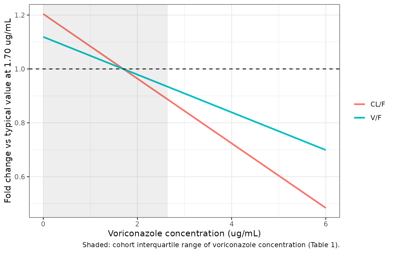
  caption = "Typical CL/F and V/F against voriconazole concentration at RBC = 3.49 x 10^12/L and PLT = 181.24 x 10^9/L (section 3.2 equations)."
)| Voriconazole (ug/mL) | CL/F (L/h) | V/F (L) | CL/F vs typical | V/F vs typical |
|---|---|---|---|---|
| 0.00 | 6.899 | 1829.945 | 1.204 | 1.119 |
| 0.95 | 6.246 | 1721.195 | 1.090 | 1.052 |
| 1.70 | 5.730 | 1635.340 | 1.000 | 1.000 |
| 2.64 | 5.084 | 1527.735 | 0.887 | 0.934 |
| 5.00 | 3.461 | 1257.576 | 0.604 | 0.769 |
Across the observed interquartile range of voriconazole (0 to 2.64 ug/mL) the typical CL/F falls from 6.9 to 5.08 L/h, about a 26% reduction. The red blood cell effect is the largest of the three over the cohort’s interquartile range: CL/F at RBC = 2.82 x 10^12/L is 1.66-fold that at 4.12 x 10^12/L. The platelet effect over its interquartile range (129 to 220 x 10^9/L) is 1.28-fold.
Structural verification against the closed form
At steady state on a q12h schedule the one-compartment
first-order-absorption model has an exact closed form. A typical patient
at the centring covariates dosed 0.5 mg q12h is solved with
ss = 1 and compared against it. The apparent half-life at
these values is 198 h, so steady state takes weeks to reach and the
steady-state solve needs a larger step budget and tight tolerances.
kaRef <- 3.09
clRef <- 5.73
vcRef <- 1635.34
doseMg <- 0.5
tau <- 12
obsT <- seq(0, tau, by = 0.25)

evSs <- dplyr::bind_rows(
  data.frame(time = 0, amt = doseMg, evid = 1L, cmt = "depot", ss = 1L, ii = tau),
  data.frame(time = obsT, amt = NA_real_, evid = 0L, cmt = "central", ss = 0L, ii = 0)
) |>
  dplyr::mutate(id = 1L, CONC_VORI_NGML = 1700, RBC = 3.49, PLT = 181.24) |>
  dplyr::arrange(time, dplyr::desc(evid))

simSs <- rxode2::rxSolve(
  typ, evSs, returnType = "data.frame",
  rtol = 1e-10, atol = 1e-12, ssRtol = 1e-10, ssAtol = 1e-12, maxsteps = 1e6
)
#> ℹ omega/sigma items treated as zero: 'etalvc', 'etalcl'

kelRef <- clRef / vcRef
closedSs <- 1000 * doseMg * kaRef / (vcRef * (kaRef - kelRef)) *
  (exp(-kelRef * simSs$time) / (1 - exp(-kelRef * tau)) -
     exp(-kaRef * simSs$time) / (1 - exp(-kaRef * tau)))

relDiff <- abs(simSs$Cc / closedSs - 1)
summary(relDiff)
#>      Min.   1st Qu.    Median      Mean   3rd Qu.      Max.
#> 4.503e-09 4.503e-09 4.504e-09 4.534e-09 4.562e-09 4.697e-09
stopifnot(max(relDiff) < 1e-5)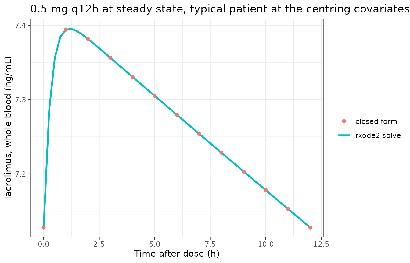
Sun 2024 does not tabulate the tacrolimus doses. At the cohort-median voriconazole concentration (0.95 ug/mL) and the centring RBC and platelet counts, the model’s average steady-state concentration equals the observed cohort median of 5.80 ng/mL at a dose of about 0.43 mg q12h. That is a low dose for tacrolimus, in line with the paper’s remark that clinicians gave patients on long-term tacrolimus smaller doses and with the CYP3A inhibition by voriconazole. The 0.5 mg q12h regimen used throughout this article is chosen on that basis; it is an illustration, not a dose from the paper.
Simulated cohort on the paper’s sampling design
Three voriconazole levels spanning the cohort distribution (0, the median 0.95 and the upper quartile 2.64 ug/mL), 100 virtual patients each, dosed 0.5 mg q12h to steady state. Red blood cell and platelet counts are drawn log-normally to match the Table 1 medians and interquartile ranges. Observation times are the union of the three sampling groups in section 2.3.1, with “30 min before the next dose” taken as 11.5 h.
# set.seed() for the base-R covariate draws, rxSetSeed() for the etas.
set.seed(20241502)
rxode2::rxSetSeed(20241502)
nPerArm <- 100L
arms <- data.frame(
  treatment = c("Cvrc 0 ug/mL", "Cvrc 0.95 ug/mL", "Cvrc 2.64 ug/mL"),
  cvrc = c(0, 0.95, 2.64)
)

# log-normal SDs from the Table 1 IQRs: (log(Q3) - log(Q1)) / 1.349
subjects <- tidyr::expand_grid(arm = seq_len(nrow(arms)), k = seq_len(nPerArm)) |>
  dplyr::mutate(
    id = dplyr::row_number(),
    treatment = arms$treatment[arm],
    cvrc = arms$cvrc[arm],
    RBC = 3.44 * exp(rnorm(dplyr::n(), 0, (log(4.12) - log(2.82)) / 1.349)),
    PLT = 170 * exp(rnorm(dplyr::n(), 0, (log(220) - log(129)) / 1.349))
  )

sampleT <- c(0, 0.5, 1, 2, 4, 6, 8, 11.5, 12)
gridT <- sort(unique(c(sampleT, seq(0, 12, by = 0.25))))

evCohort <- dplyr::bind_rows(
  subjects |>
    dplyr::mutate(time = 0, amt = doseMg, evid = 1L, cmt = "depot", ss = 1L, ii = tau),
  tidyr::expand_grid(subjects, time = gridT) |>
    dplyr::mutate(amt = NA_real_, evid = 0L, cmt = "central", ss = 0L, ii = 0)
) |>
  dplyr::mutate(CONC_VORI_NGML = cvrc * 1000) |>
  dplyr::select(id, time, amt, evid, cmt, ss, ii, CONC_VORI_NGML, RBC, PLT) |>
  dplyr::arrange(id, time, dplyr::desc(evid))

simCohort <- rxode2::rxSolve(mod, evCohort, returnType = "data.frame", maxsteps = 1e6) |>
  dplyr::left_join(dplyr::select(subjects, id, treatment), by = "id")
#> ℹ parameter labels from comments will be replaced by 'label()'

stopifnot(!anyNA(simCohort$Cc))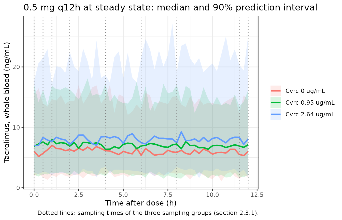
The paper’s Figure 3 VPC plots observed concentrations against an independent-variable axis of up to 600 h of clinical time with clinician-titrated doses that are not tabulated, so it cannot be regenerated without the dosing records. The cohort above shows instead what the model predicts at the paper’s sampling times for a fixed regimen.
atSamples <- simCohort |>
  dplyr::filter(time %in% sampleT[sampleT < 12]) |>
  dplyr::group_by(treatment) |>
  dplyr::summarise(
    median = median(sim),
    q25 = quantile(sim, 0.25),
    q75 = quantile(sim, 0.75),
    .groups = "drop"
  )

knitr::kable(
  atSamples |>
    dplyr::rename(
      "Arm" = treatment,
      "Median (ng/mL)" = median,
      "25th percentile" = q25,
      "75th percentile" = q75
    ),
  digits = 2,
  caption = "Simulated tacrolimus concentrations pooled over the eight sampling times, 0.5 mg q12h. Observed cohort (all doses pooled, Table 1): median 5.80 ng/mL, IQR 4.20-8.65."
)| Arm | Median (ng/mL) | 25th percentile | 75th percentile |
|---|---|---|---|
| Cvrc 0 ug/mL | 5.89 | 3.90 | 8.52 |
| Cvrc 0.95 ug/mL | 7.18 | 4.59 | 10.11 |
| Cvrc 2.64 ug/mL | 7.66 | 5.13 | 11.39 |
At the median voriconazole level the simulated spread is close to the observed Table 1 median and interquartile range. That agreement is not an independent check of the model: the regimen was chosen above so that the typical average concentration matches the observed median. What it does show is that the published inter-individual variability, together with the RBC and platelet spread, gives a concentration spread of the same width as the observed one.
PKNCA validation
Sun 2024 reports no non-compartmental analysis, so there is no published Cmax / AUC table to compare against. PKNCA is used two ways.
First, as an internal identity on the typical patient: at steady
state AUC(0-tau) = Dose / (CL/F) exactly, so PKNCA’s
dosing-interval AUC at each voriconazole level must recover the CL/F
that the section 3.2 equation gives.
evNcaTyp <- arms |>
  dplyr::mutate(id = dplyr::row_number()) |>
  dplyr::rowwise() |>
  dplyr::reframe(
    id = id, treatment = treatment, cvrc = cvrc,
    dplyr::bind_rows(
      data.frame(time = 0, amt = doseMg, evid = 1L, cmt = "depot", ss = 1L, ii = tau),
      data.frame(time = obsT, amt = NA_real_, evid = 0L, cmt = "central", ss = 0L, ii = 0)
    )
  ) |>
  dplyr::mutate(CONC_VORI_NGML = cvrc * 1000, RBC = 3.49, PLT = 181.24) |>
  dplyr::arrange(id, time, dplyr::desc(evid))

simNcaTyp <- rxode2::rxSolve(
  typ, dplyr::select(evNcaTyp, -treatment, -cvrc), returnType = "data.frame",
  rtol = 1e-10, atol = 1e-12, ssRtol = 1e-10, ssAtol = 1e-12, maxsteps = 1e6
) |>
  dplyr::left_join(dplyr::distinct(evNcaTyp, id, treatment, cvrc), by = "id")
#> ℹ omega/sigma items treated as zero: 'etalvc', 'etalcl'
#> Warning: multi-subject simulation without without 'omega'

concTyp <- simNcaTyp |>
  dplyr::filter(!is.na(Cc)) |>
  dplyr::select(id, treatment, time, Cc)
doseTyp <- concTyp |>
  dplyr::distinct(id, treatment) |>
  dplyr::mutate(time = 0, dose_mg = doseMg)

ssIntervals <- data.frame(
  start = 0, end = tau,
  cmax = TRUE, tmax = TRUE, cmin = TRUE, auclast = TRUE, cav = TRUE
)

ncaTyp <- PKNCA::pk.nca(
  PKNCA::PKNCAdata(
    PKNCA::PKNCAconc(concTyp, Cc ~ time | treatment + id),
    PKNCA::PKNCAdose(doseTyp, dose_mg ~ time | treatment + id),
    intervals = ssIntervals
  )
)

typCompare <- as.data.frame(ncaTyp) |>
  dplyr::select(treatment, PPTESTCD, PPORRES) |>
  tidyr::pivot_wider(names_from = PPTESTCD, values_from = PPORRES) |>
  dplyr::left_join(arms, by = "treatment") |>
  dplyr::mutate(
    clEquation = 5.73 * (1 + (cvrc - 1.70) * (-0.12)),
    aucExpected = 1000 * doseMg / clEquation,
    aucPctDiff = 100 * (auclast - aucExpected) / aucExpected
  )

knitr::kable(
  typCompare |>
    dplyr::select(treatment, cmax, tmax, cmin, auclast, aucExpected, aucPctDiff) |>
    dplyr::rename(
      "Arm" = treatment,
      "Cmax (ng/mL)" = cmax,
      "Tmax (h)" = tmax,
      "Cmin (ng/mL)" = cmin,
      "AUC0-12 NCA (ng/mL*h)" = auclast,
      "AUC0-12 Dose/CL" = aucExpected,
      "AUC % diff" = aucPctDiff
    ),
  digits = 3,
  caption = "Typical patient, 0.5 mg q12h at steady state: PKNCA dosing-interval AUC against Dose / (CL/F) from the section 3.2 equation."
)| Arm | Cmax (ng/mL) | Tmax (h) | Cmin (ng/mL) | AUC0-12 NCA (ng/mL*h) | AUC0-12 Dose/CL | AUC % diff |
|---|---|---|---|---|---|---|
| Cvrc 0 ug/mL | 6.150 | 1.25 | 5.911 | 72.471 | 72.475 | -0.006 |
| Cvrc 0.95 ug/mL | 6.789 | 1.25 | 6.535 | 80.050 | 80.055 | -0.006 |
| Cvrc 2.64 ug/mL | 8.328 | 1.25 | 8.042 | 98.349 | 98.354 | -0.005 |
stopifnot(
  # Linear-up/log-down trapezoids on a 0.25-h grid; measured error ~0.01%.
  max(abs(typCompare$aucPctDiff)) < 0.5,
  # Exposure rises with voriconazole, as the paper reports.
  all(diff(typCompare$auclast) > 0)
)
Second, as a per-arm summary of the simulated cohort, so the spread of steady-state exposure across the three voriconazole levels can be read directly. The PKNCA formula groups by arm.
concCohort <- simCohort |>
  dplyr::filter(!is.na(Cc)) |>
  dplyr::select(id, treatment, time, Cc)
doseCohort <- concCohort |>
  dplyr::distinct(id, treatment) |>
  dplyr::mutate(time = 0, dose_mg = doseMg)

ncaCohort <- PKNCA::pk.nca(
  PKNCA::PKNCAdata(
    PKNCA::PKNCAconc(concCohort, Cc ~ time | treatment + id),
    PKNCA::PKNCAdose(doseCohort, dose_mg ~ time | treatment + id),
    intervals = ssIntervals
  )
)

cohortNca <- as.data.frame(ncaCohort) |>
  dplyr::filter(PPTESTCD %in% c("cmax", "cmin", "auclast", "cav")) |>
  dplyr::group_by(treatment, PPTESTCD) |>
  dplyr::summarise(
    value = sprintf("%.2f [%.2f, %.2f]", median(PPORRES),
                    quantile(PPORRES, 0.25), quantile(PPORRES, 0.75)),
    .groups = "drop"
  ) |>
  tidyr::pivot_wider(names_from = PPTESTCD, values_from = value)

knitr::kable(
  cohortNca |>
    dplyr::rename(
      "Arm" = treatment,
      "AUC0-12 (ng/mL*h)" = auclast,
      "Cavg (ng/mL)" = cav,
      "Cmax (ng/mL)" = cmax,
      "Cmin (ng/mL)" = cmin
    ),
  caption = "Simulated cohort, 0.5 mg q12h at steady state: median [interquartile range] of individual NCA parameters by voriconazole level."
)| Arm | AUC0-12 (ng/mL*h) | Cavg (ng/mL) | Cmax (ng/mL) | Cmin (ng/mL) |
|---|---|---|---|---|
| Cvrc 0 ug/mL | 76.80 [55.84, 98.76] | 6.40 [4.65, 8.23] | 6.52 [4.73, 8.30] | 6.26 [4.56, 8.14] |
| Cvrc 0.95 ug/mL | 90.81 [64.21, 114.68] | 7.57 [5.35, 9.56] | 7.68 [5.53, 9.68] | 7.43 [5.15, 9.42] |
| Cvrc 2.64 ug/mL | 98.82 [77.45, 126.26] | 8.24 [6.45, 10.52] | 8.39 [6.56, 10.63] | 8.06 [6.34, 10.39] |
aucByArm <- as.data.frame(ncaCohort) |>
  dplyr::filter(PPTESTCD == "auclast") |>
  dplyr::group_by(treatment) |>
  dplyr::summarise(auc = median(PPORRES), .groups = "drop")

foldHighLow <- aucByArm$auc[aucByArm$treatment == "Cvrc 2.64 ug/mL"] /
  aucByArm$auc[aucByArm$treatment == "Cvrc 0 ug/mL"]
foldTypical <- (1 + 1.70 * 0.12) / (1 - (2.64 - 1.70) * 0.12)
c(simulated = foldHighLow, typical = foldTypical)
#> simulated   typical
#>  1.286659  1.357078

stopifnot(
  # The arms are independent cohorts, so their median AUC ratio scatters around
  # the typical-value ratio (1.36). The per-subject CL/F spread (IIV plus the
  # RBC and PLT draws) is about 46% CV, giving a log-SE of the ratio of two
  # 100-subject medians near 0.08; the bound below is about 3 SE either side.
  foldHighLow > 1.05,
  foldHighLow < 1.75
)
Assumptions and deviations
The voriconazole effect is linear and centred at 1.70 ug/mL, as printed. The section 3.2 equations give
(1 + (Cvrc - 1.70) * theta)on both CL/F and V/F. A linear covariate term can reach zero: CL/F does so at 10.03 ug/mL and V/F at 15.99 ug/mL. Those concentrations are within the assay’s linear range (0.35-11.26 ug/mL) but far above the cohort’s upper quartile of 2.64 ug/mL. The model file does not clamp the term; do not simulate it at voriconazole concentrations approaching 10 ug/mL. The centring value 1.70 is above the cohort median (0.95 ug/mL), and the RBC and PLT centring values (3.49 and 181.24) likewise differ from the Table 1 medians (3.44 and 170); all three appear to be cohort means and are used exactly as printed.Power forms for RBC and platelets. The MathML of the section 3.2
Clequation sets -1.34 and 0.46 as superscripts of(RBC/3.49)and(PLT/181.24); the authors’ manuscript supplement renders the same line with the superscripts flattened into multiplication. The exponent reading is used: the multiplicative reading would make CL/F negative.Residual error. Phoenix NLME’s additive-plus-multiplicative error model has variance
stdev0^2 + (CMultStdev * C)^2, which is nlmixr2’s defaultadd() + prop()(combined2) form.stdev0 = 0.04is taken to be in ng/mL, the unit of the observations.omega^2values are variances. Table 4 labels themomega 2 Vandomega 2 CL; they are used directly. No covariance is reported, so the random effects are independent. The bootstrap median foromega^2 CL(0.063) differs from the final estimate (0.039); the final estimate is used.Whole blood. Tacrolimus was measured with the ARCHITECT tacrolimus chemiluminescent immunoassay, a whole-blood method (section 2.3.1); the paper does not use the word “whole blood” itself.
Doses and the VPC. Tacrolimus and voriconazole doses were titrated by clinicians and are not tabulated, so Figure 3 (VPC) and Figure 2 (goodness of fit) cannot be regenerated. The 0.5 mg q12h regimen used here is chosen from the back-calculation above and is not from the paper.
Time-varying covariates. The paper does not say whether RBC, platelet count and voriconazole concentration were applied per sample or as baselines. Voriconazole was measured alongside tacrolimus and is most naturally time-varying; the model accepts all three as time-varying columns.
Errata in the source
- Male count. Section 3.1 says “comprising 38 males”; Table 1 gives 37 male (72.55%) and 14 female, which sums to 51 and is used here.
- Table 3 confidence intervals for V/F and CL/F are on a different scale from the estimates (V/F 1635.34 L with CI 1.30-1.97; CL/F 5.73 L/h with CI 0.005-0.007), consistent with Phoenix having estimated them in thousands of litres. The Table 4 bootstrap intervals (1313.12-2013.20 L and 4.65-7.07 L/h) are on the reported scale and corroborate the point estimates.
-
Table 4 bootstrap CI for
Theta Cvrc-CLis printed as -0.20 to -0.38, which does not bracket the median of -0.12; -0.038 is presumably intended. The final estimate -0.12 is unaffected. - Voriconazole units in the Discussion. The Discussion quotes the median voriconazole concentration as “0.95 [0.00, 2.64] ng/mL”; Table 1 and the assay description give ug/mL, which is used.
- Abstract wording. The Abstract calls CL the “volume of clearance rate” and omits the voriconazole effect on V/F; the Table 3 results and section 3.2 equations are followed.