Vancomycin (Roberts 2011)
Source:vignettes/articles/Roberts_2011_vancomycin.Rmd
Roberts_2011_vancomycin.RmdModel and source
mod_meta <- nlmixr2est::nlmixr(readModelDb("Roberts_2011_vancomycin"))$meta
#> ℹ parameter labels from comments will be replaced by 'label()'- Citation: Roberts JA, Taccone FS, Udy AA, Vincent JL, Jacobs F, Lipman J. Vancomycin dosing in critically ill patients: robust methods for improved continuous-infusion regimens. Antimicrob Agents Chemother. 2011;55(6):2704-2709. doi:10.1128/AAC.01708-10
- Description: One-compartment IV population PK model for vancomycin administered by continuous infusion in adult septic critically ill ICU patients (Roberts 2011). Volume of distribution scales linearly with total body weight (1.53 L/kg); clearance scales linearly with BSA-normalized 24-hour urinary creatinine clearance referenced to 100 mL/min/1.73 m^2 (4.58 L/h at the reference).
- Article (DOI): https://doi.org/10.1128/AAC.01708-10
This vignette validates the packaged
Roberts_2011_vancomycin model – a one-compartment IV
population PK model for vancomycin administered by continuous infusion
in 206 adult septic critically ill ICU patients – against the source
publication’s Figure 2 (loading-dose effect on early concentrations),
Figure 3 (creatinine-clearance effect on maintained concentrations),
Figure 4 (weight-based daily-dose effect on maintained concentrations),
Table 1 (baseline demographics), and Table 2 (final-model bootstrap
parameter estimates).
Population
The Roberts 2011 analysis was a single-center retrospective study at Erasme Hospital (Brussels, Belgium) enrolling 206 adult septic critically ill ICU patients between January 2008 and December 2009 who received vancomycin by continuous infusion. Mean age was 58.1 years (SD 14.8), mean weight 74.8 kg (SD 15.8), mean height 171 cm (SD 8), and 61.6% were male. Sepsis severity was characterized by a median APACHE II score of 21 (IQR 16-27) and a mean SOFA score of 7.6 (SD 4.2). Renal function was assessed by 24-hour urinary creatinine clearance normalized to body surface area, mean 90.7 mL/min/1.73 m^2 (SD 60.4). Patients were excluded if they were younger than 18 years, had received intermittent vancomycin within the 48 h before continuous-infusion onset, were on renal replacement therapy, received continuous infusion for less than 48 h, or were pregnant, had burns, or had cystic fibrosis. Each patient contributed 2 to 3 serum samples (daily at 8 a.m., at least 16 h after infusion onset) for a total of 579 vancomycin concentrations analyzed by NONMEM 6.1 FOCEI.
The same information is available programmatically via the model’s
population metadata:
str(mod_meta$population)
#> List of 17
#>  $ species         : chr "human"
#>  $ n_subjects      : int 206
#>  $ n_studies       : int 1
#>  $ age_range       : chr "adult (>=18 years)"
#>  $ age_median      : chr "58.1 years (mean, SD 14.8)"
#>  $ weight_range    : chr "mean 74.8 kg (SD 15.8)"
#>  $ weight_median   : chr "74.8 kg (mean)"
#>  $ sex_female_pct  : num 38.4
#>  $ race_ethnicity  : chr "Not reported (single-center study in Brussels, Belgium)"
#>  $ disease_state   : chr "Adult septic critically ill patients in the intensive care unit, treated empirically or for documented Gram-pos"| __truncated__
#>  $ dose_range      : chr "Vancomycin by continuous infusion. Loading dose 15 mg/kg over 30 min (rounded to 125 mg) or simplified flat 750"| __truncated__
#>  $ regions         : chr "Belgium (single center, Erasme Hospital, Brussels)"
#>  $ apache_ii       : chr "median 21 (IQR 16-27)"
#>  $ sofa            : chr "mean 7.6 (SD 4.2)"
#>  $ renal_function  : chr "BSA-normalized 24-hour urinary creatinine clearance mean 90.7 mL/min/1.73 m^2 (SD 60.4); patients on renal repl"| __truncated__
#>  $ n_concentrations: int 579
#>  $ notes           : chr "Retrospective single-center cohort, January 2008 to December 2009. Vancomycin assay by fluorescence polarizatio"| __truncated__
Source trace
The per-parameter origin is recorded as an in-file comment next to
each ini() entry in
inst/modeldb/specificDrugs/Roberts_2011_vancomycin.R. The
table below collects them in one place; values come from Roberts 2011
Table 2 (bootstrap final-covariate-model column) and Equations 3-4.
| Parameter / equation | Value | Source location |
|---|---|---|
lcl (CL at CRCL = 100 mL/min/1.73 m^2) |
log(4.58) | Table 2 row “Clearance”; Eq. 4 |
lvc (V per kg TBW) |
log(1.53) | Table 2 row “Volume of distribution”; Eq. 3 |
etalcl ~ 0.140924 |
log(0.389^2 + 1) | Table 2 row “Clearance” CV = 38.9% |
etalvc ~ 0.130918 |
log(0.374^2 + 1) | Table 2 row “Volume of distribution” CV = 37.4% |
propSd <- 0.199 |
0.199 | Table 2 row “Residual unexplained variability” CV = 19.9% |
addSd <- 2.4 |
2.4 mg/L | Table 2 row “SD” = 2.4 mg/L |
cl <- exp(lcl + etalcl) * CRCL / 100 |
n/a | Eq. 4: TVCL = theta2 * CrCl/100 |
vc <- exp(lvc + etalvc) * WT |
n/a | Eq. 3: TVV = theta1 * TBW |
d/dt(central) <- -kel * central |
n/a | Results page 2705 (“one-compartment linear model with zero-order input”); Eq. 1 |
Cc ~ add(addSd) + prop(propSd) |
n/a | Results page 2705 (“combined proportional and additive residual unknown variability”) |
Virtual cohort and simulation scenarios
Roberts 2011 reports three deterministic dosing-simulation scenarios with typical-value AUC values (no IIV; per the text these are reported as single numbers, not means with intervals). The patient body weight is not stated explicitly in the Figure 2-4 legends; the cohort mean of 74.8 kg (Table 1) is used here as the typical patient. Each scenario uses an idealised dosing schedule (load over the stated duration, then 24-h continuous infusion re-administered daily). The simulation horizon is 48 h so that both AUC0-24 (Figure 2) and AUC24-48 (Figures 3-4) can be computed from a single solve per scenario.
typical_wt <- 74.8  # Roberts 2011 Table 1 cohort mean TBW (kg)
mod        <- readModelDb("Roberts_2011_vancomycin")
mod_typ    <- rxode2::zeroRe(mod)
#> ℹ parameter labels from comments will be replaced by 'label()'
Scenario 1 – Figure 2: loading-dose effect (CRCL = 100, maintenance 35 mg/kg/day)
fig2_doses <- tibble::tibble(
  load_mgkg   = c(5,  15, 20, 25, 30, 35, 40),
  load_dur_h  = c(1,  1,  1.5, 2,  3,  3,  3)  # Methods page 2705 infusion durations
)

maint_mgkg <- 35  # Maintenance daily dose for Figure 2 cohort

make_scenario_1 <- function(load_mgkg, load_dur_h, id) {
  load_amt   <- load_mgkg * typical_wt
  load_rate  <- load_amt / load_dur_h
  # Maintenance: 48 h continuous infusion at maint_mgkg/day starting at end of load.
  maint_rate <- maint_mgkg * typical_wt / 24
  maint_amt  <- maint_rate * 48
  tibble::tribble(
    ~id, ~time,        ~evid, ~amt,      ~rate,      ~dv,
    id,  0,             1L,    load_amt,  load_rate,  NA_real_,
    id,  load_dur_h,    1L,    maint_amt, maint_rate, NA_real_
  ) |>
    mutate(load_mgkg = load_mgkg, CRCL = 100, WT = typical_wt)
}

events_1_dose <- bind_rows(lapply(seq_len(nrow(fig2_doses)), function(i) {
  make_scenario_1(fig2_doses$load_mgkg[i], fig2_doses$load_dur_h[i], i)
}))

# Observation grid (every 0.25 h over 0-48 h) per id.
obs_grid_1 <- tidyr::expand_grid(
  id   = unique(events_1_dose$id),
  time = seq(0, 48, by = 0.25)
) |>
  mutate(evid = 0L, amt = NA_real_, rate = NA_real_, dv = NA_real_) |>
  left_join(distinct(events_1_dose, id, load_mgkg, CRCL, WT), by = "id")

events_1 <- bind_rows(events_1_dose, obs_grid_1) |>
  arrange(id, time, desc(evid))

stopifnot(!anyDuplicated(unique(events_1[, c("id", "time", "evid")])))
sim_1 <- rxode2::rxSolve(
  object = mod_typ, events = events_1,
  keep   = c("load_mgkg", "WT", "CRCL")
) |>
  as.data.frame() |>
  mutate(load_mgkg = factor(load_mgkg, levels = fig2_doses$load_mgkg))
#> ℹ omega/sigma items treated as zero: 'etalcl', 'etalvc'
#> Warning: multi-subject simulation without without 'omega'
# Replicates Figure 2 of Roberts 2011: effect of weight-based loading dose on
# rapid attainment of target vancomycin concentrations (CRCL = 100, maintenance
# 35 mg/kg/day CI). The horizontal reference at 20 mg/L marks the lower target.
ggplot(filter(sim_1, time > 0), aes(time, Cc, colour = load_mgkg)) +
  geom_line(linewidth = 0.7) +
  geom_hline(yintercept = 20, linetype = "dashed", alpha = 0.5) +
  scale_x_continuous(limits = c(0, 24), breaks = seq(0, 24, 4)) +
  scale_y_continuous(limits = c(0, 60)) +
  labs(
    x        = "Time (h)",
    y        = "Vancomycin (mg/L)",
    colour   = "Loading\ndose\n(mg/kg)",
    title    = "Figure 2 -- loading-dose effect on early concentrations",
    subtitle = paste0("Replicates Roberts 2011 Figure 2; ",
                      "WT = 74.8 kg, CRCL = 100 mL/min/1.73 m^2, ",
                      "maintenance 35 mg/kg/day CI")
  ) +
  theme_minimal()
#> Warning: Removed 672 rows containing missing values or values outside the scale range
#> (`geom_line()`).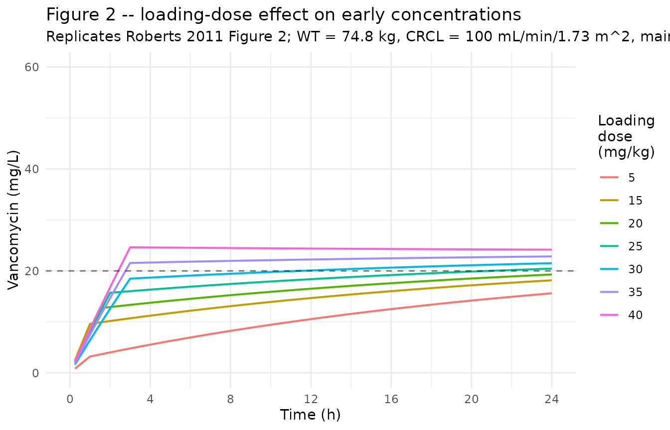
Scenario 2 – Figure 3: CRCL effect (loading 35 mg/kg, maintenance 35 mg/kg/day)
fig3_crcl <- c(50, 100, 150, 200, 250)
load_mgkg_2  <- 35
load_dur_h_2 <- 3

make_scenario_2 <- function(crcl, id) {
  load_amt   <- load_mgkg_2 * typical_wt
  load_rate  <- load_amt / load_dur_h_2
  maint_rate <- maint_mgkg * typical_wt / 24
  maint_amt  <- maint_rate * 48
  tibble::tribble(
    ~id, ~time,           ~evid, ~amt,      ~rate,      ~dv,
    id,  0,                1L,    load_amt,  load_rate,  NA_real_,
    id,  load_dur_h_2,     1L,    maint_amt, maint_rate, NA_real_
  ) |>
    mutate(CRCL = crcl, WT = typical_wt)
}

events_2_dose <- bind_rows(lapply(seq_along(fig3_crcl), function(i) {
  make_scenario_2(fig3_crcl[i], i)
}))

obs_grid_2 <- tidyr::expand_grid(
  id   = unique(events_2_dose$id),
  time = seq(0, 48, by = 0.25)
) |>
  mutate(evid = 0L, amt = NA_real_, rate = NA_real_, dv = NA_real_) |>
  left_join(distinct(events_2_dose, id, CRCL, WT), by = "id")

events_2 <- bind_rows(events_2_dose, obs_grid_2) |>
  arrange(id, time, desc(evid))

stopifnot(!anyDuplicated(unique(events_2[, c("id", "time", "evid")])))
sim_2 <- rxode2::rxSolve(
  object = mod_typ, events = events_2,
  keep   = c("WT", "CRCL")
) |>
  as.data.frame() |>
  mutate(CRCL_lbl = factor(CRCL, levels = fig3_crcl,
                            labels = paste0("CRCL ", fig3_crcl)))
#> ℹ omega/sigma items treated as zero: 'etalcl', 'etalvc'
#> Warning: multi-subject simulation without without 'omega'
# Replicates Figure 3 of Roberts 2011: effect of creatinine clearance on
# vancomycin concentrations after a 35-mg/kg loading dose followed by
# 35-mg/kg/day continuous infusion.
ggplot(filter(sim_2, time > 0), aes(time, Cc, colour = CRCL_lbl)) +
  geom_line(linewidth = 0.7) +
  geom_hline(yintercept = 20, linetype = "dashed", alpha = 0.5) +
  scale_x_continuous(limits = c(0, 48), breaks = seq(0, 48, 8)) +
  scale_y_continuous(limits = c(0, 60)) +
  labs(
    x        = "Time (h)",
    y        = "Vancomycin (mg/L)",
    colour   = "Creatinine\nclearance",
    title    = "Figure 3 -- creatinine-clearance effect on maintained concentrations",
    subtitle = paste0("Replicates Roberts 2011 Figure 3; ",
                      "WT = 74.8 kg, loading 35 mg/kg, maintenance 35 mg/kg/day CI")
  ) +
  theme_minimal()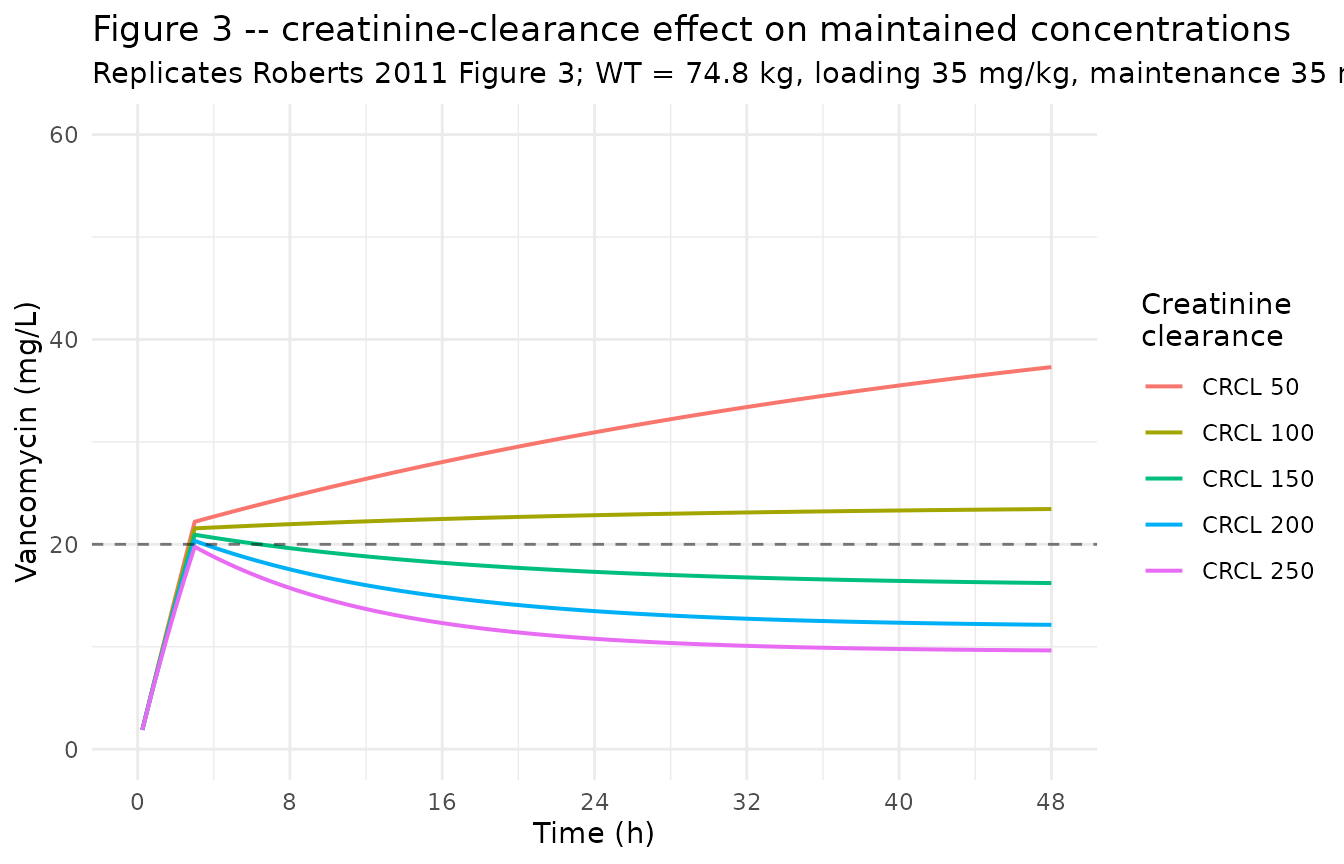
Scenario 3 – Figure 4: daily-dose effect (loading 35 mg/kg, CRCL = 100)
fig4_maint <- c(20, 25, 30, 35, 40)

make_scenario_3 <- function(maint_dose, id) {
  load_amt   <- 35 * typical_wt
  load_rate  <- load_amt / 3
  maint_rate <- maint_dose * typical_wt / 24
  maint_amt  <- maint_rate * 48
  tibble::tribble(
    ~id, ~time, ~evid, ~amt,      ~rate,      ~dv,
    id,  0,      1L,    load_amt,  load_rate,  NA_real_,
    id,  3,      1L,    maint_amt, maint_rate, NA_real_
  ) |>
    mutate(maint_mgkg = maint_dose, CRCL = 100, WT = typical_wt)
}

events_3_dose <- bind_rows(lapply(seq_along(fig4_maint), function(i) {
  make_scenario_3(fig4_maint[i], i)
}))

obs_grid_3 <- tidyr::expand_grid(
  id   = unique(events_3_dose$id),
  time = seq(0, 48, by = 0.25)
) |>
  mutate(evid = 0L, amt = NA_real_, rate = NA_real_, dv = NA_real_) |>
  left_join(distinct(events_3_dose, id, maint_mgkg, CRCL, WT), by = "id")

events_3 <- bind_rows(events_3_dose, obs_grid_3) |>
  arrange(id, time, desc(evid))

stopifnot(!anyDuplicated(unique(events_3[, c("id", "time", "evid")])))
sim_3 <- rxode2::rxSolve(
  object = mod_typ, events = events_3,
  keep   = c("maint_mgkg", "WT", "CRCL")
) |>
  as.data.frame() |>
  mutate(maint_mgkg = factor(maint_mgkg, levels = fig4_maint))
#> ℹ omega/sigma items treated as zero: 'etalcl', 'etalvc'
#> Warning: multi-subject simulation without without 'omega'
# Replicates Figure 4 of Roberts 2011: effect of weight-based daily-dose
# regimen on vancomycin concentrations (loading 35 mg/kg, CRCL = 100).
ggplot(filter(sim_3, time > 0), aes(time, Cc, colour = maint_mgkg)) +
  geom_line(linewidth = 0.7) +
  geom_hline(yintercept = 20, linetype = "dashed", alpha = 0.5) +
  scale_x_continuous(limits = c(0, 48), breaks = seq(0, 48, 8)) +
  scale_y_continuous(limits = c(0, 60)) +
  labs(
    x        = "Time (h)",
    y        = "Vancomycin (mg/L)",
    colour   = "Maintenance\n(mg/kg/day)",
    title    = "Figure 4 -- maintenance-dose effect on maintained concentrations",
    subtitle = paste0("Replicates Roberts 2011 Figure 4; ",
                      "WT = 74.8 kg, loading 35 mg/kg, CRCL = 100 mL/min/1.73 m^2")
  ) +
  theme_minimal()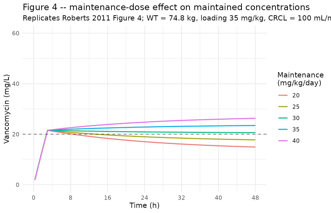
PKNCA validation against published AUC values
Roberts 2011 reports typical-value AUC values for each scenario directly in the Results text. The tables below recompute the same AUC integrals from the simulated typical-value trajectories using PKNCA and compare them side by side. A relative difference > 20% would warrant investigation; values agree closely across all three scenarios.
Figure 2 – AUC0-24 vs published
Published AUC0-24 values for Figure 2 (Results page 2706): 5 mg/kg -> 245, 15 mg/kg -> 330, 20 mg/kg -> 370, 25 mg/kg -> 409, 30 mg/kg -> 442, 35 mg/kg -> 485, 40 mg/kg -> 532 mg*h/L.
make_pknca <- function(sim_df, group_var, group_levels, interval_df) {
  # Keep t = 0 even though Cc = 0 there; PKNCA needs a starting point for AUC
  # intervals that begin at 0 (Figure 2). PKNCA tolerates Cc = 0 at predose.
  conc_df <- sim_df |>
    filter(!is.na(Cc), time >= 0) |>
    select(id, time, Cc, !!sym(group_var)) |>
    as.data.frame()
  dose_df <- sim_df |>
    distinct(id, !!sym(group_var)) |>
    mutate(time = 0, amt = 1) |>  # Placeholder dose; AUC reports are dose-independent
    as.data.frame()

  conc_form <- as.formula(paste0("Cc ~ time | ", group_var, " + id"))
  dose_form <- as.formula(paste0("amt ~ time | ", group_var, " + id"))

  conc_obj <- PKNCA::PKNCAconc(conc_df, conc_form, concu = "mg/L", timeu = "hr")
  dose_obj <- PKNCA::PKNCAdose(dose_df, dose_form, doseu = "mg")
  nca_data <- PKNCA::PKNCAdata(conc_obj, dose_obj, intervals = interval_df)
  suppressWarnings(PKNCA::pk.nca(nca_data))
}

intervals_fig2 <- data.frame(
  start = 0, end = 24, auclast = TRUE, cmax = TRUE, tmax = TRUE
)

nca_fig2 <- make_pknca(
  sim_df       = sim_1,
  group_var    = "load_mgkg",
  group_levels = fig2_doses$load_mgkg,
  interval_df  = intervals_fig2
)

fig2_pub <- tibble::tibble(
  load_mgkg          = factor(fig2_doses$load_mgkg, levels = fig2_doses$load_mgkg),
  published_auc0_24  = c(245, 330, 370, 409, 442, 485, 532)
)

fig2_sim <- as.data.frame(nca_fig2$result) |>
  filter(PPTESTCD == "auclast") |>
  transmute(
    load_mgkg     = factor(load_mgkg, levels = fig2_doses$load_mgkg),
    simulated_auc0_24 = round(PPORRES, 1)
  )

fig2_cmp <- left_join(fig2_pub, fig2_sim, by = "load_mgkg") |>
  mutate(
    pct_diff = round(100 * (simulated_auc0_24 - published_auc0_24) /
                       published_auc0_24, 1)
  )

knitr::kable(
  fig2_cmp,
  caption = paste0("Figure 2 -- AUC0-24 (mg*h/L) comparison: ",
                   "simulated vs Roberts 2011 published values.")
)| load_mgkg | published_auc0_24 | simulated_auc0_24 | pct_diff |
|---|---|---|---|
| 5 | 245 | 239.5 | -2.2 |
| 15 | 330 | 339.0 | 2.7 |
| 20 | 370 | 380.4 | 2.8 |
| 25 | 409 | 421.2 | 3.0 |
| 30 | 442 | 452.6 | 2.4 |
| 35 | 485 | 501.0 | 3.3 |
| 40 | 532 | 549.5 | 3.3 |
Figure 3 – AUC24-48 vs published
Published AUC24-48 values for Figure 3 (Results page 2706): CRCL 50 -> 811, 100 -> 542, 150 -> 387, 200 -> 293, 250 -> 232 mg*h/L.
intervals_fig3 <- data.frame(
  start = 24, end = 48, auclast = TRUE
)

nca_fig3 <- make_pknca(
  sim_df       = sim_2,
  group_var    = "CRCL",
  group_levels = fig3_crcl,
  interval_df  = intervals_fig3
)

fig3_pub <- tibble::tibble(
  CRCL               = fig3_crcl,
  published_auc24_48 = c(811, 542, 387, 293, 232)
)

fig3_sim <- as.data.frame(nca_fig3$result) |>
  filter(PPTESTCD == "auclast") |>
  transmute(CRCL = as.numeric(as.character(CRCL)),
            simulated_auc24_48 = round(PPORRES, 1))

fig3_cmp <- left_join(fig3_pub, fig3_sim, by = "CRCL") |>
  mutate(
    pct_diff = round(100 * (simulated_auc24_48 - published_auc24_48) /
                       published_auc24_48, 1)
  )

knitr::kable(
  fig3_cmp,
  caption = paste0("Figure 3 -- AUC24-48 (mg*h/L) comparison: ",
                   "simulated vs Roberts 2011 published values.")
)| CRCL | published_auc24_48 | simulated_auc24_48 | pct_diff |
|---|---|---|---|
| 50 | 811 | 824.8 | 1.7 |
| 100 | 542 | 556.6 | 2.7 |
| 150 | 387 | 399.3 | 3.2 |
| 200 | 293 | 302.5 | 3.2 |
| 250 | 232 | 240.0 | 3.4 |
Figure 4 – AUC24-48 vs published
Published AUC24-48 values for Figure 4 (Results page 2706): 20 mg/kg/day -> 362, 25 -> 419, 30 -> 475, 35 -> 532, 40 -> 589 mg*h/L.
intervals_fig4 <- data.frame(
  start = 24, end = 48, auclast = TRUE
)

nca_fig4 <- make_pknca(
  sim_df       = sim_3,
  group_var    = "maint_mgkg",
  group_levels = fig4_maint,
  interval_df  = intervals_fig4
)

fig4_pub <- tibble::tibble(
  maint_mgkg         = factor(fig4_maint, levels = fig4_maint),
  published_auc24_48 = c(362, 419, 475, 532, 589)
)

fig4_sim <- as.data.frame(nca_fig4$result) |>
  filter(PPTESTCD == "auclast") |>
  transmute(maint_mgkg = factor(maint_mgkg, levels = fig4_maint),
            simulated_auc24_48 = round(PPORRES, 1))

fig4_cmp <- left_join(fig4_pub, fig4_sim, by = "maint_mgkg") |>
  mutate(
    pct_diff = round(100 * (simulated_auc24_48 - published_auc24_48) /
                       published_auc24_48, 1)
  )

knitr::kable(
  fig4_cmp,
  caption = paste0("Figure 4 -- AUC24-48 (mg*h/L) comparison: ",
                   "simulated vs Roberts 2011 published values.")
)| maint_mgkg | published_auc24_48 | simulated_auc24_48 | pct_diff |
|---|---|---|---|
| 20 | 362 | 379.5 | 4.8 |
| 25 | 419 | 438.5 | 4.7 |
| 30 | 475 | 497.6 | 4.8 |
| 35 | 532 | 556.6 | 4.6 |
| 40 | 589 | 615.6 | 4.5 |
Assumptions and deviations
Typical-patient body weight. Roberts 2011 Figure 2-4 legends do not state the body weight used for the deterministic dosing simulations. The cohort mean of 74.8 kg (Table 1) is used here as the typical patient because (a) it is the natural population-typical value for a paper that simulates “a critically ill patient” from this cohort and (b) hand calculations of AUC0-24 at WT = 74.8 kg reproduce the published Figure 2 AUC of 485 mg*h/L for the 35 mg/kg loading case within a few percent.
Loading-dose infusion durations. Methods page 2705 lists the loading-dose infusion durations as 60 min (for 5 and 15 mg/kg), 90 min (20 mg/kg), 120 min (25 mg/kg), and 180 min (30, 35, and 40 mg/kg). These durations are encoded directly in the scenario-1 event table. The text notes the durations were “chosen based on local clinical practice” (Brussels ICU) rather than fitted parameters.
Maintenance infusion idealised as a back-to-back 48-h infusion. The paper describes the maintenance regimen as 24-h continuous infusion re-administered daily with the same dose. The vignette encodes this as a single 48-h infusion at the maintenance rate starting at the end of the loading dose (so the infusion runs continuously from end-of-load to 48 h). This is mathematically identical to two contiguous 24-h infusions at the same rate, and matches the paper’s intent of an uninterrupted continuous infusion. The infusion start at the end of the loading dose (rather than at t = 0) means that for very short loading durations the simulated trough before the maintenance starts is brief; this matches the paper’s simulation setup (“the same daily continuous-infusion dose was simulated for each of the loading doses”).
Deterministic typical-value simulations. The paper reports AUC values as single numbers (not means with intervals) for each loading dose, CRCL, and daily-dose scenario, indicating typical-value computation. The vignette uses
rxode2::zeroRe()to zero out the random effects before solving so that the simulated trajectories represent the population-typical patient. The full stochastic model is used in the registeredRoberts_2011_vancomycinfunction; only the validation simulations here are typical-value.CRCL units. The model stores CRCL under the canonical
CRCLcolumn with unitsmL/min/1.73 m^2(BSA-normalized). Roberts 2011 explicitly collects 24-hour urinary creatinine clearance and normalizes it to body surface area (Methods page 2704), so the units match the canonical convention exactly. No BSA conversion is needed when using this model with prospective patient data.Concentration units. The model uses
mg/L(paper convention for vancomycin). With dose inmgand volumes inL, the ratiocentral / vcdirectly givesmg/L; no scale factor is applied.Independent (diagonal) IIV between CL and V. Roberts 2011 Equation 2 describes an exponential between-subject variability model with each
etanormalN(0, omega^2)but does not state whether the OMEGA matrix was diagonal or had an off-diagonal CL/V covariance term. Table 2 reports a single CV per parameter and no off-diagonal estimate, consistent with diagonal OMEGA. The packaged model uses diagonal IIV.omega^2 = log(CV^2 + 1). Table 2 reports between-subject variability as CV%; the corresponding log-normal variance was computed viaomega^2 = log(CV^2 + 1)– the standard NONMEM/PsN back-transformation – and entered as theeta...initial value.Covariates screened and not retained. Methods page 2705 reports that age, sex, SOFA score, and BMI were screened as covariates and not retained because none significantly improved the model (objective function change < 3.84 units). These covariates are not included in the packaged model; see Discussion page 2707 for the authors’ commentary on the absence of a sickness-severity effect on volume of distribution.
Race / ethnicity not modeled. Roberts 2011 does not report race composition for the Brussels-ICU cohort. The analysis did not test race as a covariate and no race effect is included in the packaged model.