library(nlmixr2lib)
library(PKNCA)
#>
#> Attaching package: 'PKNCA'
#> The following object is masked from 'package:stats':
#>
#>     filter
library(dplyr)
#>
#> Attaching package: 'dplyr'
#> The following objects are masked from 'package:stats':
#>
#>     filter, lag
#> The following objects are masked from 'package:base':
#>
#>     intersect, setdiff, setequal, union
library(ggplot2)
Model and source
- Citation: Kyhl LE, Li S, Faerch KU, Soegaard B, Larsen F, Areberg J. Population pharmacokinetics of nalmefene in healthy subjects and its relation to μ-opioid receptor occupancy. Br J Clin Pharmacol. 2016 Feb;81(2):290-300. doi: 10.1111/bcp.12805. Epub 2016 Jan 27. PMID: 26483076; PMCID: PMC4833148.
- Description: Population PK model for nalmefene in healthy volunteers (Kyhl 2016): two-compartment model with first-order absorption after oral dosing, separate absorption rates for tablet and solution formulations, and a link to mu-opioid receptor occupancy.
- Article: https://doi.org/10.1111/bcp.12805
Nalmefene replication
Replicate figures 5 in the publication with a single 20 mg dose in
the fed state. Assumed the mean age, lean body mass, a tablet, and the
LC-MS/MS assay was used. The paper indicates that simulations used a
uniform age distribution of 18-80 years and LBM of
~N(56,72). Since no limits were provided for LBM in the
simulation settings, these simulation settings were not used.
dSimDose <-
  data.frame(
    ID = 1,
    AMT = 20, # dose in mg/kg # nolint: commented_code_linter.
    TIME = 0,
    EVID = 1,
    CMT = "depot"
  )
dSimObs <-
  data.frame(
    ID = 1,
    AMT = 0,
    WT = 5,
    TIME = seq(0, 24, by = 0.1),
    EVID = 0,
    CMT = "central"
  )
dSimPrep <-
  dplyr::bind_rows(dSimDose, dSimObs) |>
  dplyr::mutate(
    LBM = 56.28,
    AGE = 28,
    RIA_ASSAY = 0,
    FED = 1,
    FORM_TABLET = 1
  )
Kyhl2016Nalmefene <- readModelDb("Kyhl_2016_nalmefene")
conc_unit <- rxode2::rxode(Kyhl2016Nalmefene)$units[["concentration"]]
# Set BSV to zero for simulation to get a reproducible result
# nStud downsampled from 500 for vignette build budget; 95% PI band is visually unchanged
dSimNalmefene <- rxode2::rxSolve(Kyhl2016Nalmefene, events = dSimPrep, nStud = 100)
dSimNalmefene$Analyte <- "Nalmefene"
Plot plasma PK
Replicate figure 5 from the paper. Assuming that the “confidence bounds” are actually 95% prediction intervals.
dSimNalmefenePlot <-
  dSimNalmefene |>
  group_by(time) |>
  summarize(
    Q025_pk = quantile(sim, probs = 0.025),
    Q50_pk = quantile(sim, probs = 0.5),
    Q975_pk = quantile(sim, probs = 0.975),
    Q025_occ = quantile(e_mu_opioid, probs = 0.025),
    Q50_occ = quantile(e_mu_opioid, probs = 0.5),
    Q975_occ = quantile(e_mu_opioid, probs = 0.975)
  )

ggplot(dSimNalmefenePlot, aes(x = time, y = Q50_pk, ymin = Q025_pk, ymax = Q975_pk)) +
  geom_line() +
  labs(
    x = "Time (h)",
    y = paste0("Estimated plasma concentration (", conc_unit, ")")
  ) +
  geom_ribbon(fill = "gray") +
  geom_line() +
  scale_x_continuous(breaks = seq(0, 24, by = 5))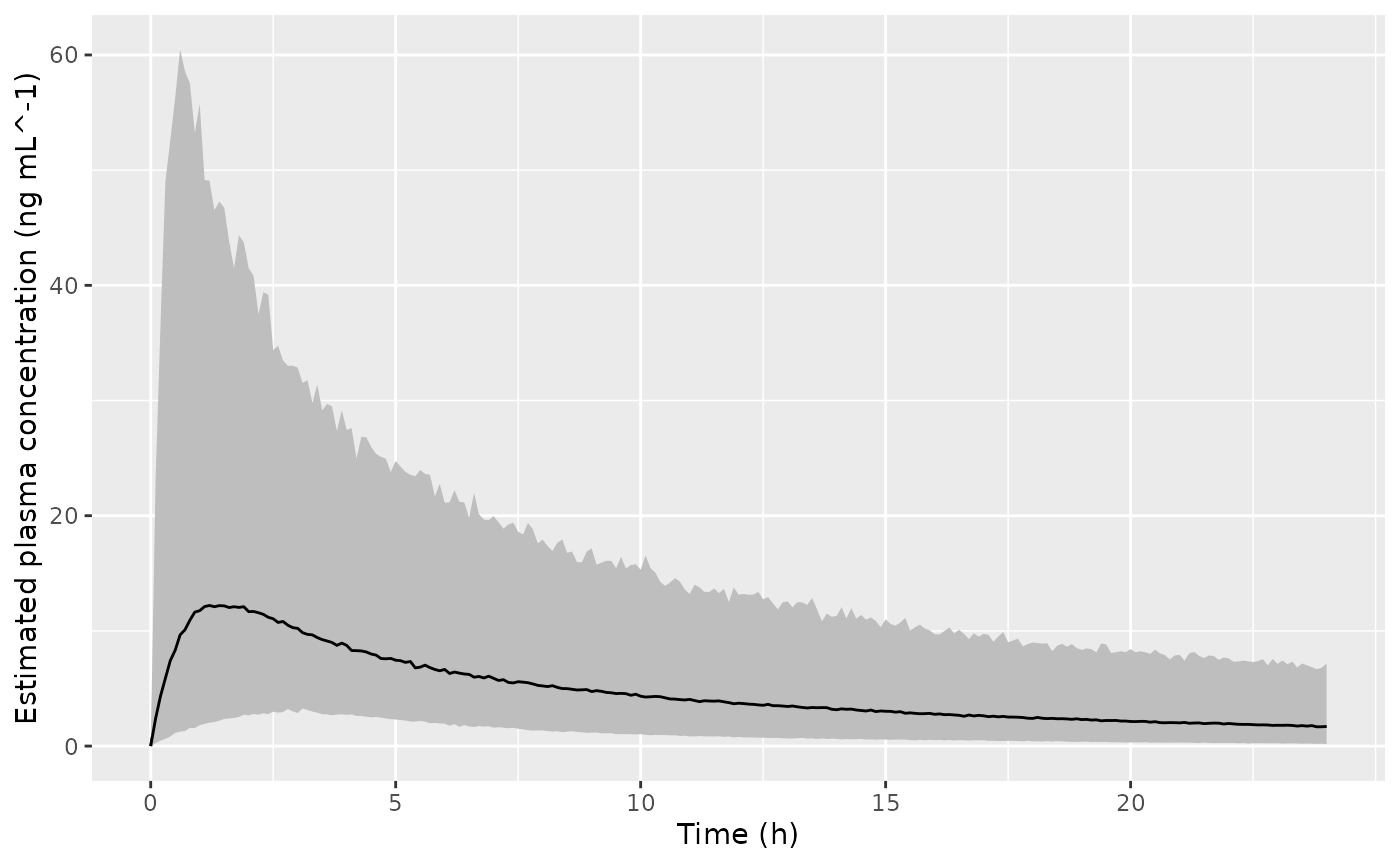
ggplot(dSimNalmefenePlot, aes(x = time, y = Q50_occ, ymin = Q025_occ, ymax = Q975_occ)) +
  geom_line() +
  labs(
    x = "Time (h)",
    y = "Occupancy (%)"
  ) +
  geom_ribbon(fill = "gray") +
  geom_line() +
  geom_hline(yintercept = c(60, 90)) +
  scale_x_continuous(breaks = seq(0, 24, by = 5))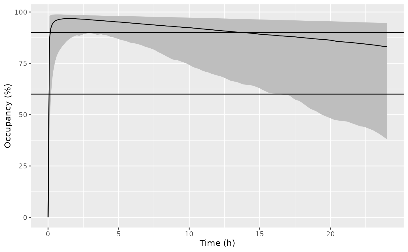
NCA analysis
Non-compartmental analysis of simulated nalmefene plasma PK (single 20 mg oral tablet in the fed state, 100 virtual subjects via IIV sampling).
# Each replicate (sim.id) is treated as an independent subject
sim_nca <- dSimNalmefene |>
  as.data.frame() |>
  mutate(treatment = "20 mg PO (fed, tablet)")

dose_nca <- sim_nca |>
  group_by(sim.id) |>
  slice(1) |>
  ungroup() |>
  mutate(time = 0, AMT = 20) |>
  select(sim.id, treatment, time, AMT)

conc_obj <- PKNCAconc(sim_nca, Cc ~ time | treatment + sim.id)
dose_obj <- PKNCAdose(dose_nca, AMT ~ time | treatment + sim.id)
data_obj <- PKNCAdata(conc_obj, dose_obj,
  intervals = data.frame(start = 0, end = 24,
                         cmax = TRUE, tmax = TRUE,
                         auclast = TRUE, half.life = TRUE))
nca_results <- pk.nca(data_obj)
nca_summary <- summary(nca_results)
knitr::kable(nca_summary, digits = 2,
caption = "NCA summary (single 20 mg oral tablet, fed state)")| start | end | treatment | N | auclast | cmax | tmax | half.life |
|---|---|---|---|---|---|---|---|
| 0 | 24 | 20 mg PO (fed, tablet) | 100 | 120 [57.5] | 15.1 [83.2] | 1.50 [0.300, 8.10] | 14.7 [10.6] |