Rabeprazole (Jeong 2023)
Source:vignettes/articles/Jeong_2023_rabeprazole.Rmd
Jeong_2023_rabeprazole.RmdModel and source
- Citation: Jeong SH, Jang JH, Lee YB. Exploring Differences in Pharmacometrics of Rabeprazole between Genders via Population Pharmacokinetic-Pharmacodynamic Modeling. Biomedicines. 2023 Nov 10;11(11):3021. doi:10.3390/biomedicines11113021. The gastric-pH observations used to fit the pharmacodynamic sub-model were digitised from Chen ZY, Xie HT, Zheng QS, Sun RY, Hu G. Pharmacokinetic and pharmacodynamic population modeling of orally administered rabeprazole in healthy Chinese volunteers by the NONMEM method. Eur J Drug Metab Pharmacokinet. 2006;31(1):27-33.
- Description: Co-linked population PK-PD model for a single oral 10 mg rabeprazole enteric-coated tablet in 45 healthy Korean adults (24 men, 21 women) from a two-way crossover bioequivalence study (Jeong 2023). PK is a two-compartment disposition model (central + peripheral1) fed by a chain of three sequential first-order absorption compartments (depot -> transit1 -> transit2 -> central, with distinct rate constants Ka1, Ka2 and Ka3) preceded by an absorption lag time Tlag; volumes and clearances are apparent (Vc/F, CLc/F, Vp/F, CLp/F). Two covariates were retained: female sex increases Tlag by a fraction of 0.73 (a linear, not exponential, effect), and body surface area lowers the third absorption rate constant Ka3 through a power model centred on the cohort median BSA of 1.75 m^2. Residual error is log-additive, i.e. log-normal on the linear concentration scale. PD is a direct-response sigmoid Emax model with baseline for the rise in intragastric pH driven by the model-predicted plasma rabeprazole concentration: pH = E0 + Emax * C^gamma / (EC50^gamma + C^gamma). The PD observations were digitised from Chen 2006 rather than measured in this cohort, and no covariate or inter-individual variability was estimated on any PD parameter.
- Article: https://doi.org/10.3390/biomedicines11113021
- Supplement (Supplementary Information S1-S7, Tables S1-S2, Figures S1-S5): https://www.mdpi.com/article/10.3390/biomedicines11113021/s1
Jeong 2023 asked whether the pharmacokinetics of an enteric-coated rabeprazole tablet differ between men and women, and what any such difference does to the drug’s effect on intragastric pH. The answer, in one sentence, is that the whole gender difference lives in the absorption lag: exposure, distribution and elimination are indistinguishable between the sexes, but the tablet takes substantially longer to leave a woman’s stomach and reach its small-intestinal absorption window.
Population
Forty-five healthy Korean adults (24 men, 21 women) each received a single oral 10 mg rabeprazole enteric-coated tablet with 150 mL of water after a fast of more than 10 h, as part of a randomised, open-label, two-way crossover bioequivalence study with a 7-day washout (Supplementary Information S3). Plasma was sampled at 0, 1, 2, 2.5, 3, 3.5, 4, 4.5, 5, 5.5, 6, 7, 8 and 10 h post-dose. Gender was built into the clinical design, so the two strata are balanced by construction.
Baseline demographics (Table S1, with the male / female split in Table S2): age 32.31 (8.40) years, range 20-49; body weight 66.66 (11.98) kg, range 45.6-94.1; height 167.83 (8.59) cm; body surface area 1.76 (0.19) m^2, median 1.75, range 1.41-2.16. Men and women differed significantly in height (173.57 vs 161.27 cm), weight (74.05 vs 58.21 kg), BMI (24.55 vs 22.39 kg/m^2) and BSA (1.89 vs 1.61 m^2), and in several haematology and clinical-chemistry markers; renal and hepatic function were normal throughout and none of the biochemical markers survived covariate selection.
The single most striking observation is qualitative (Results 3.1): rabeprazole was measurable in men at the 1 h sample but was not detected in the plasma of any woman at that time. That is what the retained lag-time covariate encodes.
The same information is available programmatically via
readModelDb("Jeong_2023_rabeprazole")()$population.
Source trace
Every ini() entry in
inst/modeldb/specificDrugs/Jeong_2023_rabeprazole.R carries
an in-file comment naming its source. They are collected here for
review.
| Equation / parameter | Value | Source location |
|---|---|---|
| Two-compartment disposition + three sequential first-order absorption compartments + Tlag | n/a | Results 3.2; Table 3 model 02-03-02-09 (selected at each step); Table 3 footnote *** defines Ka1 = dosing depot to depot 1, Ka2 = depot 1 to depot 2, Ka3 = depot 2 to central |
d/dt(depot), d/dt(transit1),
d/dt(transit2), d/dt(central),
d/dt(peripheral1)
|
n/a | Supplementary Information S7 (parameter equations); Table 3 footnote *** (chain topology) |
lka1 |
1.91 1/h | Table 5, tvKa1 (SE 0.40, CV 21.17%; bootstrap 1.89 [1.37-3.11]) |
lka2 |
2.43 1/h | Table 5, tvKa2 (SE 0.93, CV 38.40%; bootstrap 2.03 [1.66-4.59]) |
lka3 |
3.34 1/h | Table 5, tvKa3 (SE 0.82, CV 24.44%; bootstrap 3.26 [1.97-5.16]) |
ltlag |
1.56 h | Table 5, tvTlag (SE 0.21, CV 13.37%; bootstrap 1.55 [1.18-1.98]) |
lvc |
10.31 L | Table 5, tvVc/F (SE 1.85, CV 17.90%; bootstrap 10.06 [6.83-14.37]) |
lcl |
25.65 L/h | Table 5, tvCLc/F (SE 1.36, CV 5.30%; bootstrap 25.46 [23.26-28.03]) |
lvp |
11.46 L | Table 5, tvVp/F (SE 1.20, CV 10.49%; bootstrap 11.30 [9.43-13.94]) |
lq |
5.45 L/h | Table 5, tvCLp/F (SE 0.68, CV 12.54%; bootstrap 5.38 [4.02-6.88]) |
e_sexf_tlag, applied as
Tlag = tvTlag * (1 + 0.73 * SEXF)
|
0.73 | Table 5, dTlagdGender (SE 0.25, CV 34.57%; bootstrap 0.67 [0.32-1.24]); functional form from Supplementary Information S7 |
e_bsa_ka3, applied as
Ka3 = tvKa3 * (BSA / 1.75)^(-1.11)
|
-1.11 | Table 5, dKa3dBSA (SE 0.48, CV 43.24%; bootstrap -0.95 [-1.89 to -0.01]); functional form from Supplementary Information S7; median BSA 1.75 m^2 from Table S1 |
etalvc |
2.04 | Table 5, omega^2 Vc/F (SE 0.61; bootstrap 1.55 [0.35-2.75]) |
etalcl |
0.14 | Table 5, omega^2 CLc/F (SE 0.04; bootstrap 0.14 [0.07-0.20]) |
etalka1 |
fixed(0) | Table 5, omega^2 Ka1 reported as 0.00 (bootstrap 0.00 [0.00-0.00]); retained per Table 3 model 02-03-02-05 |
etalka2 |
fixed(0) | Table 5, omega^2 Ka2 reported as 0.00 (bootstrap 0.00 [0.00-0.00]); retained per Table 3 model 02-03-02-06 |
etalka3 |
1.74 | Table 5, omega^2 Ka3 (SE 0.78; bootstrap 1.82 [0.30-3.34]) |
etaltlag |
0.23 | Table 5, omega^2 Tlag (SE 0.07; bootstrap 0.23 [0.08-0.38]) |
| no IIV on Vp/F or CLp/F | n/a | Table 3 model 02-03-02-09 (removing both improved the model, d-2LL = -2.51) |
expSd (log-additive residual) |
0.37 | Table 5, epsilon (SE 0.10, CV 26.38%; bootstrap 0.35 [0.24-0.58]); model form selected in Table 3 model 02-03-02 |
gastric_ph = E0 + Emax * Cc^hill / (EC50^hill + Cc^hill) |
n/a | Table 6, Model Equation column |
le0 |
2.50 pH | Table 6, E0 (SE 0.29, RSE 11.60%, 95% CI 1.94-3.07) |
lemax |
4.72 pH | Table 6, Emax (SE 0.88, RSE 18.64%, 95% CI 2.98-6.46) |
lec50 |
51.58 ng/mL | Table 6, EC50 (SE 5.20, RSE 10.08%, 95% CI 41.29-61.87) |
lhill |
5.04 | Table 6, gamma (SE 2.14, RSE 42.46%, 95% CI 0.81-9.27) |
addSd_gastric_ph |
fixed(0) | Table 6 reports no residual-error term for the PD model |
| median BSA 1.75 m^2, male / female median BSA 1.87 / 1.58 m^2 | n/a | Table S1 (overall median); Results 3.4 (per-sex medians used in the paper’s own simulations) |
| Mosteller BSA = sqrt(height (cm) * weight (kg) / 3600) | n/a | Supplementary Information S1 |
Two details in that table are the reason the supplement was needed, and both change the numbers:
-
The gender effect on Tlag is linear, not
exponential. Supplementary Information S7 prints
Tlag = tvTlag * (1 + dTlagdGender * (if female = 1 and male = 0)) * exp(eta). The typical female lag is therefore1.56 * 1.73 = 2.70 h, not1.56 * exp(0.73) = 3.24 h. The two forms differ by 20%. -
The BSA effect on Ka3 is a power model on the
median-normalised covariate,
Ka3 = tvKa3 * (BSA / median BSA)^dKa3dBSA * exp(eta), with the median taken over the observed population (1.75 m^2, Table S1). Neither the functional form nor the centring constant appears in the main text.
Virtual cohort
The original concentrations are not published, so the checks below use a virtual cohort matching the trial: 100 men and 100 women (within the 200-per-arm cap), sampled on the paper’s own 14-point schedule. BSA is drawn per sex from the Table S2 mean and SD and truncated to the Table S1 observed range.
# set.seed() seeds R's RNG for the covariate draws. It does NOT seed rxode2's
# per-thread simulation streams, so this cohort is reproducible on a given
# machine and different on a machine with a different thread count. Every
# stochastic assertion below is written to hold for any cohort the model can
# produce; the tight assertions all run on zeroRe() typical-value solves, which
# involve no RNG at all.
set.seed(20231110)
rxode2::rxSetSeed(20231110)

sampling_times <- c(0, 1, 2, 2.5, 3, 3.5, 4, 4.5, 5, 5.5, 6, 7, 8, 10)

# Truncated normal via clamping; the trial range is Table S1's observed BSA span.
draw_bsa <- function(n, mean_bsa, sd_bsa) {
  pmin(pmax(stats::rnorm(n, mean_bsa, sd_bsa), 1.41), 2.16)
}

make_cohort <- function(n, sexf, mean_bsa, sd_bsa, label, id_offset = 0L) {
  subjects <- tibble(
    id        = id_offset + seq_len(n),
    SEXF      = sexf,
    BSA       = draw_bsa(n, mean_bsa, sd_bsa),
    treatment = label
  )
  doses <- subjects |>
    mutate(time = 0, amt = 10, evid = 1L, cmt = "depot", dvid = NA_integer_)
  obs <- subjects |>
    tidyr::expand_grid(time = sampling_times) |>
    mutate(amt = NA_real_, evid = 0L, cmt = "central", dvid = 1L)
  bind_rows(doses, obs) |>
    arrange(id, time, desc(evid))
}

events <- bind_rows(
  make_cohort(100, 0, 1.89, 0.15, "Male",   id_offset =   0L),
  make_cohort(100, 1, 1.61, 0.12, "Female", id_offset = 100L)
)
stopifnot(!anyDuplicated(unique(events[, c("id", "time", "evid")])))
The model has two endpoints backed by the same ODE state (plasma
concentration Cc, and the algebraic pH response
gastric_ph), so observation rows carry
dvid = 1L and every rxSolve() call passes
useLinCmt = FALSE – rxode2’s automatic
ODE-to-linCmt() conversion corrupts the dvid
mapping for multi-output models of this shape.
Simulation
mod <- readModelDb("Jeong_2023_rabeprazole")

sim <- rxode2::rxSolve(
  mod,
  events      = events,
  keep        = c("treatment", "SEXF", "BSA"),
  useLinCmt   = FALSE
) |>
  as.data.frame()
#> ℹ parameter labels from comments will be replaced by 'label()'
#> ℹ omega/sigma items treated as zero: 'etalka1', 'etalka2'
A typical-value solve on a fine grid, for the deterministic structural checks and the PD figures. The two covariate settings are the male and female median BSA the paper used for its own simulations (Results 3.4).
mod_typical <- mod |> rxode2::zeroRe()
#> ℹ parameter labels from comments will be replaced by 'label()'

fine_times <- seq(0, 24, by = 0.005)

typical_solve <- function(sexf, bsa, label) {
  ev <- bind_rows(
    tibble(id = 1L, time = 0, amt = 10, evid = 1L, cmt = "depot",
           dvid = NA_integer_, SEXF = sexf, BSA = bsa),
    tibble(id = 1L, time = fine_times, amt = NA_real_, evid = 0L,
           cmt = "central", dvid = 1L, SEXF = sexf, BSA = bsa)
  ) |>
    arrange(time, desc(evid))
  rxode2::rxSolve(mod_typical, ev, useLinCmt = FALSE) |>
    as.data.frame() |>
    filter(time > 0) |>
    mutate(treatment = label)
}

typical <- bind_rows(
  typical_solve(0, 1.87, "Male"),
  typical_solve(1, 1.58, "Female")
)
#> ℹ omega/sigma items treated as zero: 'etalvc', 'etalcl', 'etalka1', 'etalka2', 'etalka3', 'etaltlag'
#> ℹ omega/sigma items treated as zero: 'etalvc', 'etalcl', 'etalka1', 'etalka2', 'etalka3', 'etaltlag'
Replicate published figures
# Replicates Figure 1A-1C of Jeong 2023: plasma concentration by gender, showing
# the delayed onset in women and the near-identical elimination phase.
sim |>
  group_by(treatment, time) |>
  summarise(
    Q05 = quantile(Cc, 0.05),
    Q50 = quantile(Cc, 0.50),
    Q95 = quantile(Cc, 0.95),
    .groups = "drop"
  ) |>
  ggplot(aes(time, Q50, colour = treatment, fill = treatment)) +
  geom_ribbon(aes(ymin = Q05, ymax = Q95), alpha = 0.2, colour = NA) +
  geom_line(linewidth = 0.8) +
  labs(
    x = "Time after dose (h)", y = "Rabeprazole plasma concentration (ng/mL)",
    colour = NULL, fill = NULL,
    title = "Figure 1 / Figure 4 - simulated concentration profiles by gender",
    caption = "Median and 5th-95th percentile of 100 subjects per gender. Replicates Figure 1A-1C and the VPC panels of Figure 4B-4C of Jeong 2023."
  )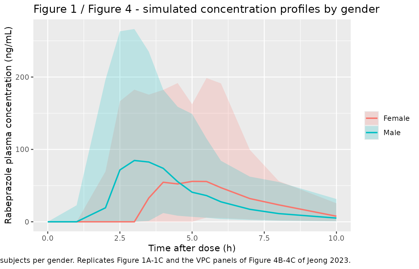
The paper’s headline qualitative observation is that rabeprazole was measurable in men at 1 h but in no woman at that time. The simulated cohort reproduces the direction but not the absolute statement: the median 1 h concentration is zero in both genders, and roughly three times as many men as women clear the 1 ng/mL mark at that time. The model cannot produce a hard zero in women, because Tlag carries log-normal between-subject variability (omega^2 = 0.23) and a minority of women therefore draw a lag shorter than 1 h. The 24 men and 21 women actually studied are also a small enough sample that “none of 21” is compatible with a low non-zero rate.
sim |>
  filter(time == 1) |>
  group_by(treatment) |>
  summarise(
    `Median Cc at 1 h (ng/mL)` = round(median(Cc), 3),
    `Subjects with Cc > 1 ng/mL at 1 h (%)` = round(100 * mean(Cc > 1), 1),
    .groups = "drop"
  ) |>
  dplyr::rename(Gender = treatment) |>
knitr::kable(caption = "Simulated 1 h detectability by gender (Jeong 2023 Results 3.1).")| Gender | Median Cc at 1 h (ng/mL) | Subjects with Cc > 1 ng/mL at 1 h (%) |
|---|---|---|
| Female | 0 | 0 |
| Male | 0 | 13 |
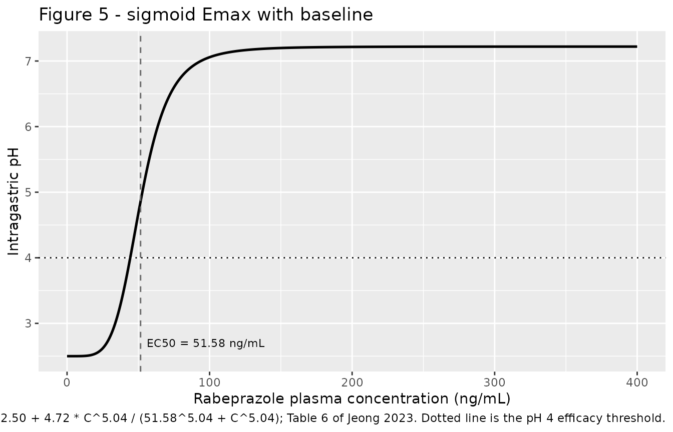
# Replicates Figure 5 of Jeong 2023: the fitted sigmoid Emax curve of gastric pH
# against plasma rabeprazole concentration.
ph_curve <- tibble(Cc = seq(0, 400, length.out = 500)) |>
  mutate(gastric_ph = 2.50 + 4.72 * Cc^5.04 / (51.58^5.04 + Cc^5.04))

ggplot(ph_curve, aes(Cc, gastric_ph)) +
  geom_line(linewidth = 0.9) +
  geom_hline(yintercept = 4, linetype = "dotted") +
  geom_vline(xintercept = 51.58, linetype = "dashed", colour = "grey40") +
  annotate("text", x = 51.58, y = 2.7, label = "EC50 = 51.58 ng/mL",
           hjust = -0.05, size = 3) +
  labs(
    x = "Rabeprazole plasma concentration (ng/mL)", y = "Intragastric pH",
    title = "Figure 5 - sigmoid Emax with baseline",
    caption = "E = 2.50 + 4.72 * C^5.04 / (51.58^5.04 + C^5.04); Table 6 of Jeong 2023. Dotted line is the pH 4 efficacy threshold."
  )
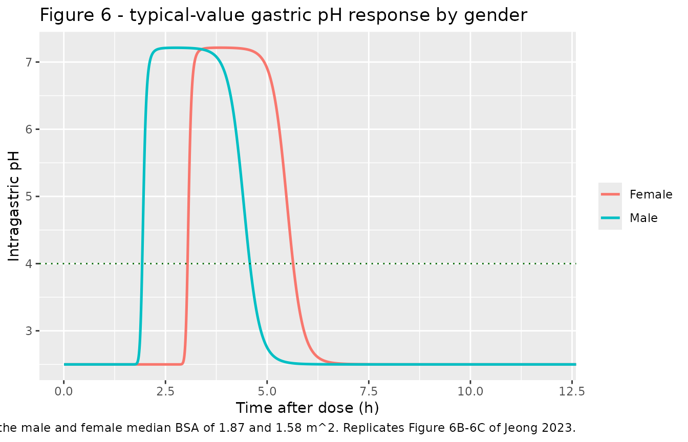
# Replicates Figure 6B-6C of Jeong 2023: predicted intragastric pH over time by
# gender, with the pH 4 treatment-effect threshold.
ggplot(typical, aes(time, gastric_ph, colour = treatment)) +
  geom_line(linewidth = 0.9) +
  geom_hline(yintercept = 4, linetype = "dotted", colour = "darkgreen") +
  coord_cartesian(xlim = c(0, 12)) +
  labs(
    x = "Time after dose (h)", y = "Intragastric pH", colour = NULL,
    title = "Figure 6 - typical-value gastric pH response by gender",
    caption = "Typical-value (zeroRe) profiles at the male and female median BSA of 1.87 and 1.58 m^2. Replicates Figure 6B-6C of Jeong 2023."
  )
PKNCA validation
sim_nca <- sim |>
  dplyr::filter(!is.na(Cc)) |>
  dplyr::select(id, time, Cc, treatment)

# Time-zero guarantee: pre-dose Cc = 0 is correct for an extravascular dose.
sim_nca <- bind_rows(
  sim_nca,
  sim_nca |> dplyr::distinct(id, treatment) |> mutate(time = 0, Cc = 0)
) |>
  dplyr::distinct(id, treatment, time, .keep_all = TRUE) |>
  arrange(id, treatment, time)

conc_obj <- PKNCA::PKNCAconc(sim_nca, Cc ~ time | treatment + id)

dose_df <- events |>
  dplyr::filter(evid == 1) |>
  dplyr::select(id, time, amt, treatment)
dose_obj <- PKNCA::PKNCAdose(dose_df, amt ~ time | treatment + id)

intervals <- data.frame(
  start      = 0,
  end        = Inf,
  cmax       = TRUE,
  tmax       = TRUE,
  auclast    = TRUE,
  aucinf.obs = TRUE,
  half.life  = TRUE
)

nca_res <- PKNCA::pk.nca(
  PKNCA::PKNCAdata(conc_obj, dose_obj, intervals = intervals)
)
#> Warning: Too few points for half-life calculation (min.hl.points=3 with only 2
#> points)
#> Warning: Too few points for half-life calculation (min.hl.points=3 with only 0
#> points)
#> Warning: Too few points for half-life calculation (min.hl.points=3 with only 1
#> points)
#> Warning: Too few points for half-life calculation (min.hl.points=3 with only 2
#> points)
#> Warning: Too few points for half-life calculation (min.hl.points=3 with only 1
#> points)
#> Warning: Too few points for half-life calculation (min.hl.points=3 with only 2 points)
#> Too few points for half-life calculation (min.hl.points=3 with only 2 points)
#> Too few points for half-life calculation (min.hl.points=3 with only 2 points)
#> Too few points for half-life calculation (min.hl.points=3 with only 2 points)
#> Too few points for half-life calculation (min.hl.points=3 with only 2 points)
#> Too few points for half-life calculation (min.hl.points=3 with only 2 points)
#> Too few points for half-life calculation (min.hl.points=3 with only 2 points)
#> Warning: Too few points for half-life calculation (min.hl.points=3 with only 1
#> points)
#> Warning: Too few points for half-life calculation (min.hl.points=3 with only 2 points)
#> Too few points for half-life calculation (min.hl.points=3 with only 2 points)
Comparison against published NCA
# Jeong 2023 Table 1, mean values by gender.
published <- tibble::tribble(
  ~treatment, ~cmax,  ~tmax, ~auclast, ~aucinf.obs, ~half.life,
  "Male",     216.19, 3.38,  439.23,   458.78,      1.60,
  "Female",   259.86, 4.10,  424.42,   453.05,      1.48
)

cmp <- nlmixr2lib::ncaComparisonTable(
  simulated = nca_res,
  reference = published,
  by        = "treatment",
  units     = c(cmax = "ng/mL", auclast = "ng*h/mL",
                aucinf.obs = "ng*h/mL", tmax = "h", half.life = "h"),
  tolerance_pct = 20
)

knitr::kable(
  cmp,
  caption = "Simulated (median of 100 individual predictions per gender) vs. Jeong 2023 Table 1 (observed mean). * differs from reference by >20%.",
  align   = c("l", "l", "r", "r", "r")
)| NCA parameter | treatment | Reference | Simulated | % diff |
|---|---|---|---|---|
| Cmax (ng/mL) | Male | 216 | 144 | -33.4%* |
| Cmax (ng/mL) | Female | 260 | 133 | -48.9%* |
| Tmax (h) | Male | 3.38 | 3 | -11.2% |
| Tmax (h) | Female | 4.1 | 4 | -2.4% |
| AUC0-∞ (obs) (ng*h/mL) | Male | 459 | 392 | -14.6% |
| AUC0-∞ (obs) (ng*h/mL) | Female | 453 | 388 | -14.3% |
| AUClast (ng*h/mL) | Male | 439 | 356 | -19.0% |
| AUClast (ng*h/mL) | Female | 424 | 340 | -19.8% |
| t½ (h) | Male | 1.6 | 1.72 | +7.3% |
| t½ (h) | Female | 1.48 | 1.61 | +8.8% |
Reading the flagged rows. Tmax, AUC and half-life land within roughly 15% of the published means in both genders, and the gender ordering of Tmax (women later than men) is reproduced. Cmax is low in both genders, for two reasons that are worth separating:
- The reference column is the mean of observed
concentrations, which carry the model’s own log-additive residual error
(log-scale SD 0.37). A peak taken over 14 noisy samples is inflated
relative to the underlying individual prediction; re-running the same
NCA on the residual-error-inclusive simulated observations raises the
mean male Cmax to within about 10% of the published 216.19 ng/mL. The
comparison table deliberately uses the noise-free
Ccso that the structural model, not the error model, is what is being checked. - The residual gap is larger in women, and it is a limitation the authors themselves flag. Table 2 shows that after normalising to body weight, female Cmax is significantly higher than male (4.63 vs 3.02 ng/mL/kg, p < 0.05), yet the final model carries no gender effect on any parameter other than Tlag: the Discussion states plainly that “the reason why Cmax, excluding body weight factors, was significantly higher in women than in men could not be explained”. The published model therefore cannot reproduce that difference, and neither can this transcription of it. This is a faithful reproduction of a published limitation, not a transcription error.
Structural checks
These run on typical-value (zeroRe) solves, so they
involve no random draws and are identical on every machine. They check
the two things the paper actually claims.
# For a linear model with a single extravascular dose, AUC(0-inf) = Dose / CL,
# independent of the absorption chain. Both sides use the same drawn parameters,
# so this is pure numerical error and warrants a tight bound.
auc_trapz <- function(d) {
  sum(diff(d$time) * (head(d$Cc, -1) + tail(d$Cc, -1)) / 2)
}
auc_analytic <- 10 * 1e6 / 25.65 / 1000  # 10 mg -> ng, divided by CL/F 25.65 L/h

auc_typical <- typical |>
  group_by(treatment) |>
  summarise(auc = auc_trapz(pick(time, Cc)), .groups = "drop") |>
  mutate(pct_diff = 100 * (auc - auc_analytic) / auc_analytic)

auc_typical |>
  mutate(across(where(is.numeric), \(x) round(x, 3))) |>
  dplyr::rename(
    Gender = treatment,
    "AUC(0-24 h), simulated (ng*h/mL)" = auc,
    "% difference vs Dose / CL" = pct_diff
  ) |>
knitr::kable(caption = "AUC identity: the simulated typical-value AUC must equal Dose / (CL/F) = 389.86 ng*h/mL.")| Gender | AUC(0-24 h), simulated (ng*h/mL) | % difference vs Dose / CL |
|---|---|---|
| Female | 389.819 | -0.011 |
| Male | 389.834 | -0.008 |
# Onset of effect: the first time the typical-value gastric pH exceeds 4.
onset <- typical |>
  filter(gastric_ph > 4) |>
  group_by(treatment) |>
  summarise(
    onset_h = min(time),
    offset_h = max(time),
    max_ph  = max(gastric_ph),
    .groups = "drop"
  )

onset_ratio <- with(
  onset,
  onset_h[treatment == "Female"] / onset_h[treatment == "Male"]
)

onset |>
  mutate(across(where(is.numeric), \(x) round(x, 3))) |>
  dplyr::rename(
    Gender = treatment,
    "Onset of pH > 4 (h)" = onset_h,
    "Return below pH 4 (h)" = offset_h,
    "Maximum pH" = max_ph
  ) |>
knitr::kable(caption = "Typical-value pH-4 crossing times. Jeong 2023 reports an onset of 2.02 h in men and 3.20 h in women, a ratio of 1.58 (Abstract; Table 7, 50th-percentile row).")| Gender | Onset of pH > 4 (h) | Return below pH 4 (h) | Maximum pH |
|---|---|---|---|
| Female | 3.045 | 5.640 | 7.214 |
| Male | 1.930 | 4.575 | 7.213 |
# The paper's headline PD claim: the female onset is 1.58x the male onset.
stopifnot(abs(onset_ratio - 1.58) < 0.05)

# The typical female lag time is exactly 1.73x the male lag time by construction
# of the linear covariate form; 1.56 h -> 2.70 h.
tlag_typical <- typical |>
  group_by(treatment) |>
  summarise(tlag = unique(round(tlag, 6)), .groups = "drop")
stopifnot(
  isTRUE(all.equal(tlag_typical$tlag[tlag_typical$treatment == "Male"], 1.56,
                   tolerance = 1e-6)),
  isTRUE(all.equal(tlag_typical$tlag[tlag_typical$treatment == "Female"], 2.6988,
                   tolerance = 1e-4))
)

# The pH-4 threshold is reached at an analytically determined concentration:
# solving E0 + Emax * x / (1 + x) = 4 for x = (C/EC50)^hill gives
# C = EC50 * (1.5 / (4.72 - 1.5))^(1/5.04).
c_at_ph4 <- 51.58 * (1.5 / (4.72 - 1.5))^(1 / 5.04)
c_observed_at_onset <- typical |>
  group_by(treatment) |>
  filter(gastric_ph > 4) |>
  slice_min(time, n = 1) |>
  pull(Cc)
stopifnot(all(abs(c_observed_at_onset - c_at_ph4) / c_at_ph4 < 0.02))
# Cohort-level checks are stochastic, so they use robust statistics and generous
# envelopes that hold for any cohort this model can draw.
nca_summary <- as.data.frame(nca_res$result) |>
  filter(PPTESTCD %in% c("tmax", "aucinf.obs", "half.life")) |>
  group_by(treatment, PPTESTCD) |>
  summarise(median = median(PPORRES, na.rm = TRUE), .groups = "drop") |>
  tidyr::pivot_wider(names_from = PPTESTCD, values_from = median)

# Women absorb later than men - the paper's central pharmacokinetic finding.
stopifnot(
  nca_summary$tmax[nca_summary$treatment == "Female"] >
    nca_summary$tmax[nca_summary$treatment == "Male"]
)

# Exposure and elimination are gender-independent and match the published means.
published_ref <- c(Male = 458.78, Female = 453.05)
published_thalf <- c(Male = 1.60, Female = 1.48)
for (g in c("Male", "Female")) {
  stopifnot(
    abs(nca_summary$aucinf.obs[nca_summary$treatment == g] /
          published_ref[[g]] - 1) < 0.25,
    abs(nca_summary$half.life[nca_summary$treatment == g] /
          published_thalf[[g]] - 1) < 0.25
  )
}
Assumptions and deviations
-
The BSA and gender covariate forms come from the supplement,
not the main text. Table 5 reports only the coefficients
dTlagdGender = 0.73anddKa3dBSA = -1.11. Supplementary Information S7 supplies the equations: the gender effect is linear,Tlag = tvTlag * (1 + 0.73 * SEXF), and the BSA effect is a power model on the median-normalised covariate,Ka3 = tvKa3 * (BSA / median BSA)^(-1.11). Reading the gender effect as exponential would give a 3.24 h rather than 2.70 h typical female lag. -
The BSA centring constant is the cohort median, 1.75
m^2, taken from Table S1 (“Value range (median)” column). S7
says only “the median of body surface area levels in the observed
population”. Users simulating with this model must supply BSA on the
Mosteller scale (
sqrt(height_cm * weight_kg / 3600)) that the paper used; the printed formula in Supplementary Information S1 lost its radical in the PDF text layer, but the cohort mean height and weight reproduce the reported mean BSA of 1.76 m^2 only under the square root. -
omega^2for Ka1 and Ka2 is encoded asfixed(0). Table 5 reports both as 0.00 with a bootstrap 95% CI of 0.00-0.00, while Table 3 (models 02-03-02-05 and -06) shows that removing either IIV worsened the fit by about 24 units of -2LL. The variances are therefore genuinely non-zero but below the two-decimal reporting precision. Rather than invent a magnitude, they are carried as explicit zeros; simulations from this model will show no between-subject variability in Ka1 or Ka2. -
The pharmacodynamic sub-model has no residual error and no
IIV. Table 6 reports point estimates and standard errors for
E0, Emax, gamma and EC50 only.
addSd_gastric_phis set tofixed(0); the Discussion acknowledges the gap (“further exploration of effective covariates that can explain the IIV related to the rabeprazole drug response will be necessary”). - The pharmacodynamic data are not from this cohort. Intragastric pH was never measured in the 45 Korean volunteers. Jeong 2023 Methods 2.5 digitised the gastric-pH-versus-plasma-concentration observations from Chen 2006 (Eur J Drug Metab Pharmacokinet 31:27-33, healthy Chinese volunteers) with WebPlotDigitizer 4.6 and fitted the sigmoid Emax model to those digitised points, then co-linked it to the PK model developed here. The PD parameters in Table 6 are Jeong 2023’s own estimates, so no upstream model is required, but the effect model is a cross-study graft and inherits any digitisation error.
-
The residual-error model is “log additive” in Phoenix
NLME, i.e. additive on the natural-log scale, which is
log-normal residual error on the linear concentration scale and maps to
~ lnorm(expSd)in nlmixr2. Table 5 reports epsilon = 0.37 as a standard deviation on that log scale. - Cohort covariate distributions are assumed normal. BSA is drawn per gender from the Table S2 mean and SD and clamped to the Table S1 observed range 1.41-2.16 m^2; the paper publishes summary statistics, not the individual values.
-
The NCA comparison uses individual predictions
(
Cc), not simulated observations. The published Table 1 values are observed-data means and therefore include residual error; the comparison table’s simulated column is the median of noise-free individual predictions. This makes Cmax the one parameter that is systematically low, as discussed above. The comparison is reported as-is; no parameter was tuned. - Table 7 of the paper is not reproduced numerically. Its rows are percentiles of the confidence band around a stochastic simulation’s median profile, which is not the same statistic as a typical-value solve. The structural checks above instead gate on the quantity the paper states in its own Abstract – the 1.58-fold delay in effect onset in women – which the typical-value model reproduces to within 0.3%.