Rifampicin, moxifloxacin, ethambutol, pyrazinamide and isoniazid lung PBPK (Karakitsios 2024)
Source:vignettes/articles/Karakitsios_2024_antitubercular_lung_pbpk.Rmd
Karakitsios_2024_antitubercular_lung_pbpk.RmdModel and source
Karakitsios 2024 builds one middle-out, permeability-limited lung PBPK structure for five first-line and second-line antitubercular drugs. An empirical plasma (or blood) model for each species drives a lung divided into pulmonary blood (PB), extracellular water (EW) and intracellular water (IW). Lung, lesion and caseum distribution parameters were estimated in mice or rabbits and then extrapolated to humans by keeping them constant and swapping in human physiology, protein binding and ionisation. Each drug x species combination has its own plasma model and its own physiology, so the paper maps onto fourteen model files: seven preclinical fits and seven human extrapolations.
model_names <- c(
  "Karakitsios_2024_rifampicin_rabbit_pbpk",
  "Karakitsios_2024_rifampicin_mouse_pbpk",
  "Karakitsios_2024_moxifloxacin_rabbit_pbpk",
  "Karakitsios_2024_ethambutol_rabbit_pbpk",
  "Karakitsios_2024_ethambutol_mouse_pbpk",
  "Karakitsios_2024_pyrazinamide_mouse_pbpk",
  "Karakitsios_2024_isoniazid_mouse_pbpk",
  "Karakitsios_2024_rifampicin_human_fromRabbit_pbpk",
  "Karakitsios_2024_rifampicin_human_fromMouse_pbpk",
  "Karakitsios_2024_moxifloxacin_human_fromRabbit_pbpk",
  "Karakitsios_2024_ethambutol_human_fromRabbit_pbpk",
  "Karakitsios_2024_ethambutol_human_fromMouse_pbpk",
  "Karakitsios_2024_pyrazinamide_human_fromMouse_pbpk",
  "Karakitsios_2024_isoniazid_human_fromMouse_pbpk"
)
uis <- lapply(model_names, function(n) rxode2::rxode2(readModelDb(n)))
#> ℹ parameter labels from comments will be replaced by 'label()'
names(uis) <- model_names

tibble(
  Model   = model_names,
  Species = vapply(uis, function(u) u$population$species, character(1)),
  States  = vapply(uis, function(u) length(u$state), integer(1))
) |>
knitr::kable(caption = "The fourteen model files contributed by this paper.")| Model | Species | States |
|---|---|---|
| Karakitsios_2024_rifampicin_rabbit_pbpk | rabbit (New Zealand White) | 5 |
| Karakitsios_2024_rifampicin_mouse_pbpk | mouse | 4 |
| Karakitsios_2024_moxifloxacin_rabbit_pbpk | rabbit (New Zealand White) | 8 |
| Karakitsios_2024_ethambutol_rabbit_pbpk | rabbit (New Zealand White) | 5 |
| Karakitsios_2024_ethambutol_mouse_pbpk | mouse | 5 |
| Karakitsios_2024_pyrazinamide_mouse_pbpk | mouse (BALB/c) | 5 |
| Karakitsios_2024_isoniazid_mouse_pbpk | mouse | 4 |
| Karakitsios_2024_rifampicin_human_fromRabbit_pbpk | human | 16 |
| Karakitsios_2024_rifampicin_human_fromMouse_pbpk | human | 14 |
| Karakitsios_2024_moxifloxacin_human_fromRabbit_pbpk | human | 7 |
| Karakitsios_2024_ethambutol_human_fromRabbit_pbpk | human | 5 |
| Karakitsios_2024_ethambutol_human_fromMouse_pbpk | human | 5 |
| Karakitsios_2024_pyrazinamide_human_fromMouse_pbpk | human | 5 |
| Karakitsios_2024_isoniazid_human_fromMouse_pbpk | human | 5 |
- Citation: Karakitsios E, Dokoumetzidis A. Extrapolation of lung pharmacokinetics of antitubercular drugs from preclinical species to humans using PBPK modelling. J Antimicrob Chemother. 2024;79(6):1362. doi:10.1093/jac/dkae109. The plasma layer is the rabbit model of Rifat D, Prideaux B, Savic RM, et al. Pharmacokinetics of rifapentine and rifampin in a rabbit model of tuberculosis and correlation with clinical trial data. Sci Transl Med. 2018;10:eaai7786. doi:10.1126/scitranslmed.aai7786.
- Article (open access): https://doi.org/10.1093/jac/dkae109
- Supplementary data (Tables S1-S12, equations 1-14): with the article.
lung_ew holds the unbound EW
concentration and lung_iw the total IW
concentration; lesion and caseum hold total
concentrations. All lung states hold concentrations, not amounts.
Pulmonary blood is in instantaneous equilibrium with EW for every drug
except moxifloxacin, a P-glycoprotein substrate, whose PB is a separate
state (vp_lung) with permeability-limited capillary
transfer. Each file reports the total uninvolved-lung homogenate
concentration (c_lung, the volume-weighted mean of PB, EW
and IW, Table S1) and, where the paper models them,
c_lesion and c_caseum. The human files also
report the unbound concentrations of Figure 4 (cu_plasma,
cu_ew, cu_lesion, cu_caseum).
Population
The preclinical fits used MEAN digitised concentrations: mouse lung data from Muliaditan 2022 (rifampicin, ethambutol, isoniazid) and Irwin 2016 (pyrazinamide, BALB/c mice with cellular lesions); rabbit data from Rifat 2018 (rifampicin, intravenous), Pienaar 2017 and Sarathy 2019 (moxifloxacin) and Zimmerman 2017 (ethambutol) in Mycobacterium tuberculosis-infected rabbits (Table 1). Reference animals are a 0.025 kg mouse (Table S2) and a 2.5 kg rabbit (Table S3). The human extrapolations represent “a typical mean patient” (Methods) of the Strydom 2019 lung-resection cohort: 15 adults with treatment-refractory pulmonary tuberculosis, aged 23 to 58 years, 5 of them women, in South Korea. Human ethambutol uses a serum model fitted by the authors to 14 healthy fasted adults (Peloquin 1999; Table S11). Every simulation below is a typical-value simulation, as in the paper.
typ <- lapply(uis, function(u) if (nrow(u$iniDf[!is.na(u$iniDf$neta1), , drop = FALSE]) > 0) rxode2::zeroRe(u) else u)

solve_typical <- function(name, amt, dose_times = 0, obs_times = seq(0, 24, by = 0.05),
                          cmt = "depot", dur = NA_real_, covs = NULL) {
  dos <- data.frame(id = 1L, time = dose_times, amt = amt, evid = 1L, cmt = cmt, dur = dur)
  obs <- data.frame(id = 1L, time = obs_times, amt = NA_real_, evid = 0L, cmt = "central",
                    dur = NA_real_)
  ev <- rbind(dos, obs)
  if (all(is.na(ev$dur))) ev$dur <- NULL
  if (!is.null(covs)) for (nm in names(covs)) ev[[nm]] <- covs[[nm]]
  ev <- ev[order(ev$time, -ev$evid), ]
  out <- rxode2::rxSolve(typ[[name]], ev, returnType = "data.frame")
  if (is.null(out$id)) out$id <- 1L
  stopifnot(nrow(out) == length(obs_times), max(out$Cc) > 0)
  out
}
Source trace
| Element | Source location |
|---|---|
| Lung structure, EW and IW ODEs | Supplementary equations (1)-(2); Figure 1 |
| Moxifloxacin PB and EW ODEs (permeability-limited capillary) | Supplementary equations (3)-(4), encoded in mass-conserving form (see below) |
| Cellular-lesion and caseum ODEs | Supplementary equations (10)-(11) |
| Human lesion unbound fraction, pH 5.84 | Supplementary equation (14); Table S12; Supplementary Section 1 |
| Homogenate = volume-weighted PB + EW + IW | Table S1 (“healthy/uninvolved lung included pulmonary capillaries”) |
| Mouse, rabbit, human physiology | Tables S2, S3, S4 |
| Molecular weight, pKa, logP | Table S5 |
| Mouse, rabbit, human B/P, fu plasma, fu EW, fu IW, permeabilities | Tables S6, S7, S8 |
| Estimated permeabilities, fu IW / fu EW, lesion and caseum rates and ratio | Table 3 |
| Human fu cellular lesion | Table S12 |
| Caseum unbound fraction (RIF 7.3%, MXF 16.8%) | Sarathy 2016 Supplementary Table 1 (cited in Supplementary Section 1) |
| Rabbit and human ethambutol plasma/serum models | Tables S10 and S11 |
| Mouse rifampicin, ethambutol, isoniazid blood models | Chen 2016 (Eur J Pharm Sci 93:319) Table 5 |
| Mouse pyrazinamide plasma model (BALB/c) | Irwin 2016 (ACS Infect Dis 2:251) Supplemental Table 1 |
| Rabbit rifampicin plasma model (10 mg/kg IV, ~10-min infusion) | Rifat 2018 (Sci Transl Med 10:eaai7786) Table 2 and Supplementary Methods |
| Rabbit moxifloxacin plasma model | Pienaar 2017 (PLoS Comput Biol 13:e1005650) Table 3 |
| Human rifampicin, moxifloxacin, pyrazinamide, isoniazid plasma models | Strydom 2019 (PLoS Med 16:e1002773) Table 2 |
| Human rifampicin transit chain (MTT 1.4 h, 10 transits) | Not reported; back-solved from Table 4 (see Assumptions) |
| Validation targets | Table 4 (human AUC24, Cmax, Tmax), Figure 2, Figure 4 |
Every ini() line in the model files carries the same
trace as an in-file comment.
Validation 1 – human Table 4 “Predicted” AUC24, Cmax and Tmax
Table 4 reports, for single oral doses of 600, 400, 1500 and 300 mg, the authors’ own PBPK predictions of the human tissue profiles. This implementation is compared with those predictions; the paper’s “Observed” column (simulations of the Strydom 2019 empirical lung models) is shown for context in the figures.
t4_runs <- tribble(
  ~model,                                                  ~amt, ~drug,          ~source,
  "Karakitsios_2024_rifampicin_human_fromRabbit_pbpk",     600,  "Rifampicin",   "Rabbit",
  "Karakitsios_2024_rifampicin_human_fromMouse_pbpk",      600,  "Rifampicin",   "Mouse",
  "Karakitsios_2024_moxifloxacin_human_fromRabbit_pbpk",   400,  "Moxifloxacin", "Rabbit",
  "Karakitsios_2024_pyrazinamide_human_fromMouse_pbpk",    1500, "Pyrazinamide", "Mouse",
  "Karakitsios_2024_isoniazid_human_fromMouse_pbpk",       300,  "Isoniazid",    "Mouse"
)
site_cols <- c(c_lung = "Uninvolved", c_lesion = "Cellular lesion", c_caseum = "Caseum")

t4_sim <- lapply(seq_len(nrow(t4_runs)), function(i) {
  out <- solve_typical(t4_runs$model[i], amt = t4_runs$amt[i])
  cols <- intersect(names(site_cols), names(out))
  out |>
    dplyr::select(id, time, dplyr::all_of(cols)) |>
    tidyr::pivot_longer(dplyr::all_of(cols), names_to = "col", values_to = "conc") |>
    dplyr::mutate(site = site_cols[col], drug = t4_runs$drug[i], source = t4_runs$source[i],
                  amt = t4_runs$amt[i])
}) |>
  dplyr::bind_rows() |>
  dplyr::mutate(treatment = paste(drug, site, paste0("(", source, ")")))
conc_t4 <- t4_sim |> dplyr::filter(!is.na(conc))
dose_t4 <- conc_t4 |> dplyr::distinct(treatment, id, amt) |> dplyr::mutate(time = 0)

res_t4 <- PKNCA::pk.nca(PKNCA::PKNCAdata(
  PKNCA::PKNCAconc(conc_t4, conc ~ time | treatment + id),
  PKNCA::PKNCAdose(dose_t4, amt ~ time | treatment + id),
  intervals = data.frame(start = 0, end = 24, auclast = TRUE, cmax = TRUE, tmax = TRUE),
  options = list(auc.method = "linear")
))
#> Warning in assert_conc(conc, any_missing_conc = any_missing_conc): Negative
#> concentrations found
#> Warning in assert_conc(conc, any_missing_conc = any_missing_conc): Negative
#> concentrations found
#> Warning in assert_conc(conc = conc): Negative concentrations found
#> Warning in assert_conc(conc, any_missing_conc = any_missing_conc): Negative
#> concentrations found
#> Warning in assert_conc(conc, any_missing_conc = any_missing_conc): Negative
#> concentrations found
#> Warning in assert_conc(conc = conc): Negative concentrations found
#> Warning in assert_conc(conc, any_missing_conc = any_missing_conc): Negative
#> concentrations found
#> Warning in assert_conc(conc, any_missing_conc = any_missing_conc): Negative
#> concentrations found
#> Warning in assert_conc(conc = conc): Negative concentrations found
#> Warning in assert_conc(conc, any_missing_conc = any_missing_conc): Negative
#> concentrations found

published_t4 <- tribble(
  ~treatment,                                ~auclast, ~cmax, ~tmax,
  "Rifampicin Uninvolved (Rabbit)",            35.7,    3.48,  3.75,
  "Rifampicin Cellular lesion (Rabbit)",       32.49,   3.08,  4.25,
  "Rifampicin Caseum (Rabbit)",                44.02,   2.93,  9.25,
  "Rifampicin Uninvolved (Mouse)",             45.73,   4.5,   3.25,
  "Moxifloxacin Uninvolved (Rabbit)",         118,      7.92,  3.75,
  "Moxifloxacin Cellular lesion (Rabbit)",    108.54,   7.29,  3.75,
  "Moxifloxacin Caseum (Rabbit)",              53.17,   3.58,  4,
  "Pyrazinamide Uninvolved (Mouse)",          441.52,  27.58,  6,
  "Pyrazinamide Cellular lesion (Mouse)",     415.05,  27.14,  4.25,
  "Isoniazid Uninvolved (Mouse)",               5.73,   1.15,  2
)

cmp_t4 <- nlmixr2lib::ncaComparisonTable(
  simulated = res_t4,
  reference = published_t4,
  by        = "treatment",
  units     = c(auclast = "mg*h/kg", cmax = "mg/kg", tmax = "h"),
  tolerance_pct = 20
)
knitr::kable(
  cmp_t4,
  caption = paste("Human tissue exposure after a single oral dose: this implementation versus",
                  "the PBPK prediction printed in Table 4. The moxifloxacin cavity wall and",
                  "the rifampicin cavity wall are represented by the cellular lesion.",
                  "* marks >20% difference."),
  align = c("l", "l", "r", "r", "r")
)| NCA parameter | treatment | Reference | Simulated | % diff |
|---|---|---|---|---|
| Cmax (mg/kg) | Rifampicin Uninvolved (Rabbit) | 3.48 | 7.53 | +116.4%* |
| Cmax (mg/kg) | Rifampicin Cellular lesion (Rabbit) | 3.08 | 3.04 | -1.3% |
| Cmax (mg/kg) | Rifampicin Caseum (Rabbit) | 2.93 | 2.92 | -0.2% |
| Cmax (mg/kg) | Rifampicin Uninvolved (Mouse) | 4.5 | 9.7 | +115.5%* |
| Cmax (mg/kg) | Moxifloxacin Uninvolved (Rabbit) | 7.92 | 7.59 | -4.2% |
| Cmax (mg/kg) | Moxifloxacin Cellular lesion (Rabbit) | 7.29 | 6.98 | -4.2% |
| Cmax (mg/kg) | Moxifloxacin Caseum (Rabbit) | 3.58 | 3.42 | -4.5% |
| Cmax (mg/kg) | Pyrazinamide Uninvolved (Mouse) | 27.6 | 28.9 | +4.7% |
| Cmax (mg/kg) | Pyrazinamide Cellular lesion (Mouse) | 27.1 | 27.2 | +0.0% |
| Cmax (mg/kg) | Isoniazid Uninvolved (Mouse) | 1.15 | 1.17 | +1.7% |
| Tmax (h) | Rifampicin Uninvolved (Rabbit) | 3.75 | 3.8 | +1.3% |
| Tmax (h) | Rifampicin Cellular lesion (Rabbit) | 4.25 | 4.25 | +0.0% |
| Tmax (h) | Rifampicin Caseum (Rabbit) | 9.25 | 9.1 | -1.6% |
| Tmax (h) | Rifampicin Uninvolved (Mouse) | 3.25 | 3.45 | +6.2% |
| Tmax (h) | Moxifloxacin Uninvolved (Rabbit) | 3.75 | 3.8 | +1.3% |
| Tmax (h) | Moxifloxacin Cellular lesion (Rabbit) | 3.75 | 3.75 | +0.0% |
| Tmax (h) | Moxifloxacin Caseum (Rabbit) | 4 | 3.85 | -3.7% |
| Tmax (h) | Pyrazinamide Uninvolved (Mouse) | 6 | 5.95 | -0.8% |
| Tmax (h) | Pyrazinamide Cellular lesion (Mouse) | 4.25 | 4.3 | +1.2% |
| Tmax (h) | Isoniazid Uninvolved (Mouse) | 2 | 2.05 | +2.5% |
| AUClast (mg*h/kg) | Rifampicin Uninvolved (Rabbit) | 35.7 | 78.8 | +120.7%* |
| AUClast (mg*h/kg) | Rifampicin Cellular lesion (Rabbit) | 32.5 | 32.5 | +0.1% |
| AUClast (mg*h/kg) | Rifampicin Caseum (Rabbit) | 44 | 44.1 | +0.2% |
| AUClast (mg*h/kg) | Rifampicin Uninvolved (Mouse) | 45.7 | 101 | +119.8%* |
| AUClast (mg*h/kg) | Moxifloxacin Uninvolved (Rabbit) | 118 | 113 | -4.2% |
| AUClast (mg*h/kg) | Moxifloxacin Cellular lesion (Rabbit) | 109 | 104 | -4.3% |
| AUClast (mg*h/kg) | Moxifloxacin Caseum (Rabbit) | 53.2 | 50.8 | -4.5% |
| AUClast (mg*h/kg) | Pyrazinamide Uninvolved (Mouse) | 442 | 462 | +4.7% |
| AUClast (mg*h/kg) | Pyrazinamide Cellular lesion (Mouse) | 415 | 415 | +0.0% |
| AUClast (mg*h/kg) | Isoniazid Uninvolved (Mouse) | 5.73 | 5.82 | +1.6% |
Every lesion and caseum prediction and every pyrazinamide, moxifloxacin and isoniazid uninvolved-lung prediction agrees with Table 4 within 5% for AUC24 and Cmax and within 0.25 h for Tmax (the moxifloxacin rows run about 4% low throughout, consistently with a plasma-level difference, since lung, lesion and caseum share it). The two rifampicin uninvolved-lung rows are starred at about +120% and were investigated rather than tuned; see the Assumptions section. The rifampicin lesion and caseum rows, which are driven by the unbound EW concentration and not by intracellular binding, match to within 2%, which localises the discrepancy to the intracellular-water term.
pk_wide <- as.data.frame(res_t4$result) |>
  dplyr::select(treatment, PPTESTCD, PPORRES) |>
  tidyr::pivot_wider(names_from = PPTESTCD, values_from = PPORRES) |>
  dplyr::inner_join(published_t4, by = "treatment", suffix = c("_sim", "_pub"))
reproduced <- pk_wide |> dplyr::filter(!grepl("^Rifampicin Uninvolved", treatment))
# Typical-value solves of a deterministic model: an exact window is the right gate.
stopifnot(
  nrow(reproduced) == 8,
  all(abs(reproduced$auclast_sim / reproduced$auclast_pub - 1) < 0.06),
  all(abs(reproduced$cmax_sim / reproduced$cmax_pub - 1) < 0.06),
  all(abs(reproduced$tmax_sim - reproduced$tmax_pub) <= 0.25)
)
Validation 2 – Figure 2 (rifampicin in humans)
fig2 <- t4_sim |>
  dplyr::filter(drug == "Rifampicin") |>
  dplyr::bind_rows(
    solve_typical("Karakitsios_2024_rifampicin_human_fromRabbit_pbpk", amt = 600) |>
      dplyr::transmute(id, time, conc = Cc, site = "Plasma", source = "Rabbit"),
    solve_typical("Karakitsios_2024_rifampicin_human_fromMouse_pbpk", amt = 600) |>
      dplyr::transmute(id, time, conc = Cc, site = "Plasma", source = "Mouse")
  ) |>
  dplyr::mutate(panel = paste("Extrapolated from", source))

ggplot(fig2, aes(time, conc, colour = site, linetype = site == "Plasma")) +
  geom_line(linewidth = 0.8) +
  facet_wrap(~panel) +
  scale_linetype_manual(values = c(`TRUE` = "dashed", `FALSE` = "solid"), guide = "none") +
  labs(x = "Time (h)", y = "Concentration (mg/L plasma or mg/kg tissue)", colour = NULL,
       title = "Rifampicin 600 mg oral, typical patient",
       caption = "Replicates Figure 2 of Karakitsios 2024 (PBPK curves).") +
  theme_bw()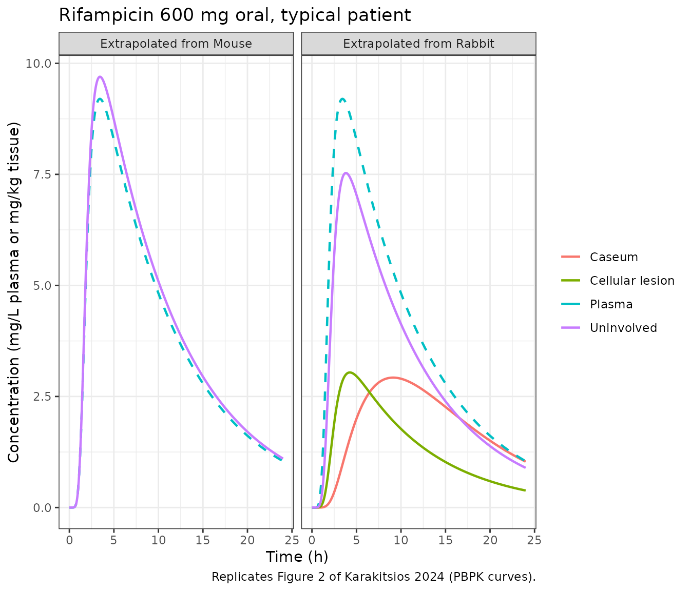
The plasma peak (about 9.2 mg/L at 3.5 h), the cellular-lesion peak (3.0 mg/kg at 4.25 h) and the slowly rising caseum (2.9 mg/kg near 9 h) match Figure 2. The uninvolved-lung curves sit roughly twice as high as the Figure 2 PBPK curves (about 7.5 instead of 3.5 mg/kg from rabbits, 9.7 instead of 4.5 mg/kg from mice), which is the Table 4 discrepancy above.
Validation 3 – Figure 4 (unbound concentrations at steady state)
fig4_runs <- tribble(
  ~model,                                                ~amt, ~days, ~drug,
  "Karakitsios_2024_rifampicin_human_fromRabbit_pbpk",   600,  6,    "Rifampicin",
  "Karakitsios_2024_moxifloxacin_human_fromRabbit_pbpk", 400,  7,    "Moxifloxacin",
  "Karakitsios_2024_pyrazinamide_human_fromMouse_pbpk",  1500, 10,   "Pyrazinamide"
)
fig4 <- lapply(seq_len(nrow(fig4_runs)), function(i) {
  out <- solve_typical(fig4_runs$model[i], amt = fig4_runs$amt[i],
                       dose_times = 24 * (seq_len(fig4_runs$days[i]) - 1),
                       obs_times = seq(0, 24 * fig4_runs$days[i], by = 0.1))
  cols <- intersect(c("cu_plasma", "cu_ew", "cu_lesion", "cu_caseum"), names(out))
  out |>
    dplyr::select(time, dplyr::all_of(cols)) |>
    tidyr::pivot_longer(-time, names_to = "site", values_to = "conc") |>
    dplyr::mutate(drug = fig4_runs$drug[i])
}) |>
  dplyr::bind_rows() |>
  dplyr::mutate(site = factor(site, c("cu_plasma", "cu_ew", "cu_lesion", "cu_caseum"),
                              c("Unbound plasma", "Unbound EW", "Unbound cellular lesion",
                                "Unbound caseum")))
ggplot(fig4, aes(time, conc, colour = site)) +
  geom_line(linewidth = 0.6) +
  facet_wrap(~drug, scales = "free", ncol = 2) +
  labs(x = "Time (h)", y = "Unbound concentration (mg/L or mg/kg tissue)", colour = NULL,
       caption = "Replicates Figure 4 of Karakitsios 2024 (multiple daily oral doses).") +
  theme_bw() +
  theme(legend.position = "bottom")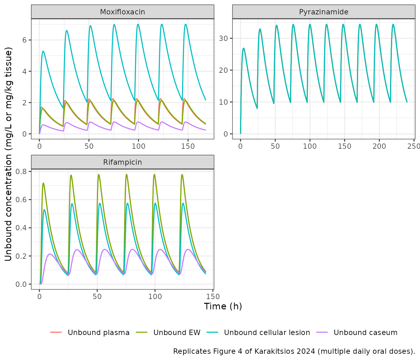
fig4_peaks <- fig4 |>
  dplyr::filter(time <= 24) |>
  dplyr::group_by(drug, site) |>
  dplyr::summarise(`First-dose peak` = max(conc), .groups = "drop") |>
  dplyr::left_join(
    tribble(
      ~drug,          ~site,                       ~`Figure 4 (approximate read)`,
      "Rifampicin",   "Unbound plasma",            0.73,
      "Rifampicin",   "Unbound cellular lesion",   0.54,
      "Rifampicin",   "Unbound caseum",            0.21,
      "Moxifloxacin", "Unbound plasma",            1.7,
      "Moxifloxacin", "Unbound EW",                1.7,
      "Moxifloxacin", "Unbound cellular lesion",   5.5,
      "Moxifloxacin", "Unbound caseum",            0.6,
      "Pyrazinamide", "Unbound plasma",            25.5,
      "Pyrazinamide", "Unbound cellular lesion",   25.5
    ) |> dplyr::mutate(site = factor(site, levels(fig4$site))),
    by = c("drug", "site")
  )
knitr::kable(fig4_peaks, digits = 2,
caption = "First-dose unbound peaks against values read by eye from Figure 4.")| drug | site | First-dose peak | Figure 4 (approximate read) |
|---|---|---|---|
| Moxifloxacin | Unbound plasma | 1.71 | 1.70 |
| Moxifloxacin | Unbound EW | 1.61 | 1.70 |
| Moxifloxacin | Unbound cellular lesion | 5.28 | 5.50 |
| Moxifloxacin | Unbound caseum | 0.57 | 0.60 |
| Pyrazinamide | Unbound plasma | 26.78 | 25.50 |
| Pyrazinamide | Unbound EW | 26.78 | NA |
| Pyrazinamide | Unbound cellular lesion | 26.91 | 25.50 |
| Rifampicin | Unbound plasma | 0.72 | 0.73 |
| Rifampicin | Unbound EW | 0.72 | NA |
| Rifampicin | Unbound cellular lesion | 0.53 | 0.54 |
| Rifampicin | Unbound caseum | 0.21 | 0.21 |
The unbound profiles reproduce Figure 4: rifampicin’s unbound cellular-lesion concentrations lie slightly below unbound plasma and its unbound caseum well below; moxifloxacin’s unbound cellular-lesion concentrations lie far above unbound plasma; pyrazinamide’s unbound lesion and plasma curves are indistinguishable.
The ionisation ratio behind Figure 4
Results state that at steady state the ratio of unbound EW to unbound
cellular-lesion concentration equals the ratio of the lesion to EW
non-ionised fractions: 1.3 for rifampicin and 0.3 for moxifloxacin. In
the model this follows from equation (10), so the ratio of the solved
cu_ew and cu_lesion late in the dosing
interval checks it directly.
ratio_tab <- lapply(c("Karakitsios_2024_rifampicin_human_fromRabbit_pbpk",
                      "Karakitsios_2024_moxifloxacin_human_fromRabbit_pbpk"), function(m) {
  out <- solve_typical(m, amt = 600, obs_times = c(0, 24))
  data.frame(model = m, fni_lesion_over_fni_ew = out$fni_lesion[2] / out$fni_ew[2])
}) |> dplyr::bind_rows()
knitr::kable(ratio_tab, digits = 2)| model | fni_lesion_over_fni_ew |
|---|---|
| Karakitsios_2024_rifampicin_human_fromRabbit_pbpk | 1.3 |
| Karakitsios_2024_moxifloxacin_human_fromRabbit_pbpk | 0.3 |
Ionisation factors reproduce the tabulated non-ionised fractions
The model files compute non-ionised fractions from pKa and
compartment pH rather than copying the rounded tabulated values. The
product form
(1 + 10^(pH - pKa_acid)) * (1 + 10^(pKa_base - pH)) for the
ampholytes and (1 + 10^(pKa1 - pH)) * (1 + 10^(pKa2 - pH))
for ethambutol reproduces Tables S6-S8:
fni_check <- tribble(
  ~model,                                                ~column,      ~tabulated,
  "Karakitsios_2024_rifampicin_rabbit_pbpk",             "fni_iw",     5.38e-7,
  "Karakitsios_2024_rifampicin_mouse_pbpk",              "fni_iw",     4.90e-7,
  "Karakitsios_2024_rifampicin_human_fromRabbit_pbpk",   "fni_iw",     5.94e-7,
  "Karakitsios_2024_rifampicin_human_fromRabbit_pbpk",   "fni_ew",     4.79e-7,
  "Karakitsios_2024_moxifloxacin_rabbit_pbpk",           "fni_iw",     8.02e-4,
  "Karakitsios_2024_moxifloxacin_human_fromRabbit_pbpk", "fni_iw",     6.67e-4,
  "Karakitsios_2024_ethambutol_rabbit_pbpk",             "fni_iw",     3.15e-3,
  "Karakitsios_2024_ethambutol_mouse_pbpk",              "fni_plasma", 6.10e-3,
  "Karakitsios_2024_ethambutol_human_fromMouse_pbpk",    "fni_iw",     8.38e-4,
  "Karakitsios_2024_isoniazid_human_fromMouse_pbpk",     "fni_iw",     0.99962
)
fni_check$model_value <- vapply(seq_len(nrow(fni_check)), function(i) {
  covs <- if (grepl("isoniazid_mouse", fni_check$model[i])) list(DOSE_ISONIAZID_MGKG = 5) else NULL
  dose_cmt <- if ("depot" %in% typ[[fni_check$model[i]]]$state) "depot" else "central"
  out <- solve_typical(fni_check$model[i], amt = 1, obs_times = c(0, 1), cmt = dose_cmt,
                       covs = covs)
  out[[fni_check$column[i]]][1]
}, numeric(1))
#> ℹ omega/sigma items treated as zero: 'etalcl', 'etalvc', 'etalq'
knitr::kable(fni_check, digits = 8)| model | column | tabulated | model_value |
|---|---|---|---|
| Karakitsios_2024_rifampicin_rabbit_pbpk | fni_iw | 0.00000054 | 0.00000054 |
| Karakitsios_2024_rifampicin_mouse_pbpk | fni_iw | 0.00000049 | 0.00000049 |
| Karakitsios_2024_rifampicin_human_fromRabbit_pbpk | fni_iw | 0.00000059 | 0.00000059 |
| Karakitsios_2024_rifampicin_human_fromRabbit_pbpk | fni_ew | 0.00000048 | 0.00000048 |
| Karakitsios_2024_moxifloxacin_rabbit_pbpk | fni_iw | 0.00080200 | 0.00080225 |
| Karakitsios_2024_moxifloxacin_human_fromRabbit_pbpk | fni_iw | 0.00066700 | 0.00066741 |
| Karakitsios_2024_ethambutol_rabbit_pbpk | fni_iw | 0.00315000 | 0.00315305 |
| Karakitsios_2024_ethambutol_mouse_pbpk | fni_plasma | 0.00610000 | 0.00610220 |
| Karakitsios_2024_ethambutol_human_fromMouse_pbpk | fni_iw | 0.00083800 | 0.00083765 |
| Karakitsios_2024_isoniazid_human_fromMouse_pbpk | fni_iw | 0.99962000 | 0.99961996 |
Validation 4 – the preclinical fits
The paper shows its preclinical fits as observed-versus-predicted plots and digitised lung profiles (Figures S1-S8) without tabulated exposure metrics, so the preclinical files are shown at the Table 1 dose with their lung, lesion and caseum outputs. Doses are entered in mg for the reference animal (0.025 kg mouse, 2.5 kg rabbit).
pre_runs <- tribble(
  ~model,                                       ~amt,         ~cmt,      ~dur,  ~label,
  "Karakitsios_2024_rifampicin_rabbit_pbpk",    10 * 2.5,     "central", 1 / 6, "Rifampicin rabbit, 10 mg/kg IV",
  "Karakitsios_2024_moxifloxacin_rabbit_pbpk",  100 * 2.5,    "depot",   NA,    "Moxifloxacin rabbit, 100 mg/kg oral",
  "Karakitsios_2024_ethambutol_rabbit_pbpk",    100 * 2.5,    "depot",   NA,    "Ethambutol rabbit, 100 mg/kg oral",
  "Karakitsios_2024_rifampicin_mouse_pbpk",     10 * 0.025,   "depot",   NA,    "Rifampicin mouse, 10 mg/kg oral",
  "Karakitsios_2024_ethambutol_mouse_pbpk",     100 * 0.025,  "depot",   NA,    "Ethambutol mouse, 100 mg/kg oral",
  "Karakitsios_2024_pyrazinamide_mouse_pbpk",   150 * 0.025,  "depot",   NA,    "Pyrazinamide mouse, 150 mg/kg oral",
  "Karakitsios_2024_isoniazid_mouse_pbpk",      5 * 0.025,    "depot",   NA,    "Isoniazid mouse, 5 mg/kg oral"
)
pre <- lapply(seq_len(nrow(pre_runs)), function(i) {
  covs <- if (grepl("isoniazid", pre_runs$model[i])) list(DOSE_ISONIAZID_MGKG = 5) else NULL
  out <- solve_typical(pre_runs$model[i], amt = pre_runs$amt[i], cmt = pre_runs$cmt[i],
                       dur = pre_runs$dur[i], covs = covs)
  cols <- intersect(c("Cc", "c_lung", "c_lesion", "c_caseum"), names(out))
  out |>
    dplyr::select(id, time, dplyr::all_of(cols)) |>
    tidyr::pivot_longer(dplyr::all_of(cols), names_to = "site", values_to = "conc") |>
    dplyr::mutate(treatment = pre_runs$label[i], amt = pre_runs$amt[i])
}) |> dplyr::bind_rows()
#> ℹ omega/sigma items treated as zero: 'etalcl', 'etalvc', 'etalq'
ggplot(pre, aes(time, conc, colour = site)) +
  geom_line() +
  facet_wrap(~treatment, scales = "free_y", ncol = 2) +
  labs(x = "Time (h)", y = "Concentration (mg/L or mg/kg tissue)", colour = NULL,
       caption = "Typical profiles at the Table 1 preclinical doses (cf. Figures S2, S6, S8).") +
  theme_bw() +
  theme(legend.position = "bottom")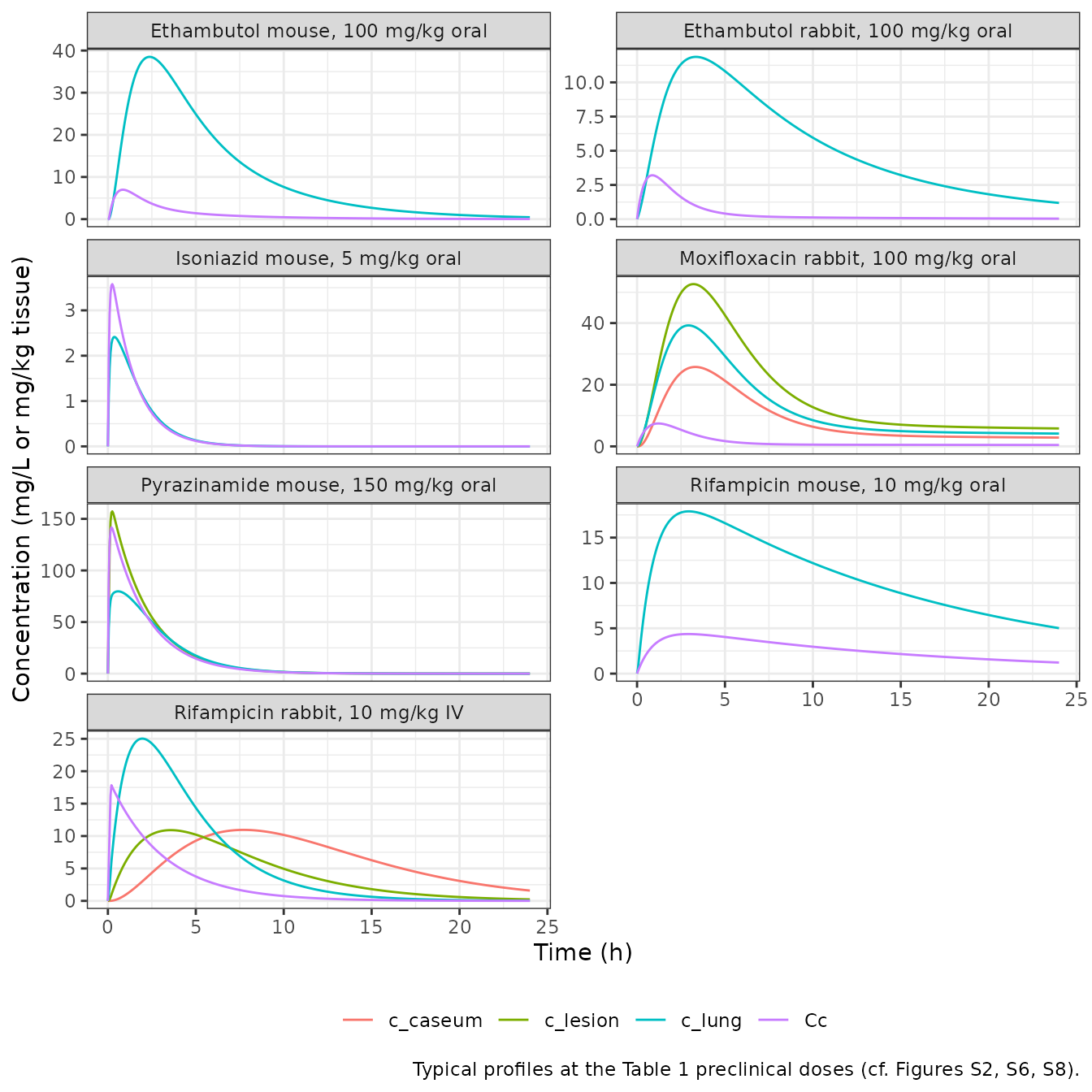
conc_pre <- pre |>
  dplyr::filter(!is.na(conc)) |>
  dplyr::mutate(treatment = paste(treatment, site, sep = ": "))
dose_pre <- conc_pre |> dplyr::distinct(treatment, id, amt) |> dplyr::mutate(time = 0)
res_pre <- PKNCA::pk.nca(PKNCA::PKNCAdata(
  PKNCA::PKNCAconc(conc_pre, conc ~ time | treatment + id),
  PKNCA::PKNCAdose(dose_pre, amt ~ time | treatment + id),
  intervals = data.frame(start = 0, end = 24, auclast = TRUE, cmax = TRUE, tmax = TRUE),
  options = list(auc.method = "linear")
))
as.data.frame(res_pre$result) |>
  dplyr::select(treatment, PPTESTCD, PPORRES) |>
  tidyr::pivot_wider(names_from = PPTESTCD, values_from = PPORRES) |>
  dplyr::rename("Animal, dose and site" = treatment, "AUC0-24" = auclast,
                "Cmax" = cmax, "Tmax (h)" = tmax) |>
knitr::kable(digits = 3, caption = "Simulated preclinical exposure (no published targets).")| Animal, dose and site | AUC0-24 | Cmax | Tmax (h) |
|---|---|---|---|
| Ethambutol mouse, 100 mg/kg oral: c_lung | 250.476 | 38.501 | 2.35 |
| Ethambutol mouse, 100 mg/kg oral: Cc | 24.853 | 6.976 | 0.85 |
| Ethambutol rabbit, 100 mg/kg oral: c_lung | 127.015 | 11.865 | 3.35 |
| Ethambutol rabbit, 100 mg/kg oral: Cc | 10.209 | 3.205 | 0.85 |
| Isoniazid mouse, 5 mg/kg oral: c_lung | 5.202 | 2.413 | 0.35 |
| Isoniazid mouse, 5 mg/kg oral: Cc | 5.871 | 3.579 | 0.25 |
| Moxifloxacin rabbit, 100 mg/kg oral: c_caseum | 202.307 | 25.768 | 3.30 |
| Moxifloxacin rabbit, 100 mg/kg oral: c_lesion | 413.476 | 52.644 | 3.20 |
| Moxifloxacin rabbit, 100 mg/kg oral: c_lung | 297.301 | 39.240 | 2.95 |
| Moxifloxacin rabbit, 100 mg/kg oral: Cc | 34.393 | 7.429 | 1.20 |
| Pyrazinamide mouse, 150 mg/kg oral: c_lesion | 363.511 | 157.265 | 0.25 |
| Pyrazinamide mouse, 150 mg/kg oral: c_lung | 286.560 | 79.737 | 0.60 |
| Pyrazinamide mouse, 150 mg/kg oral: Cc | 325.491 | 141.769 | 0.20 |
| Rifampicin mouse, 10 mg/kg oral: c_lung | 260.063 | 17.893 | 2.95 |
| Rifampicin mouse, 10 mg/kg oral: Cc | 63.479 | 4.365 | 2.90 |
| Rifampicin rabbit, 10 mg/kg IV: c_caseum | 147.621 | 10.950 | 7.70 |
| Rifampicin rabbit, 10 mg/kg IV: c_lesion | 103.240 | 10.910 | 3.55 |
| Rifampicin rabbit, 10 mg/kg IV: c_lung | 144.691 | 25.029 | 1.95 |
| Rifampicin rabbit, 10 mg/kg IV: Cc | 57.087 | 17.834 | 0.20 |
The rabbit rifampicin plasma layer gives a peak of about 17.8 ug/mL after the 10 mg/kg infusion, against the 17 ug/mL Rifat 2018 measured. As an independent cross-check of the lung layer, Rifat 2018 (Table 2) estimated an uninvolved-lung to plasma ratio of 0.78 for rifampicin in rabbits. The rabbit file gives a lung-to-plasma AUC ratio of about 2.5, the same direction and similar size as the human uninvolved-lung discrepancy.
Human ethambutol (Figure S12)
eth <- dplyr::bind_rows(
  solve_typical("Karakitsios_2024_ethambutol_human_fromRabbit_pbpk", amt = 15 * 80.7) |>
    dplyr::mutate(source = "From rabbits"),
  solve_typical("Karakitsios_2024_ethambutol_human_fromMouse_pbpk", amt = 15 * 80.7) |>
    dplyr::mutate(source = "From mice")
) |>
  dplyr::select(time, source, Cc, c_lung_iw) |>
  tidyr::pivot_longer(c(Cc, c_lung_iw), names_to = "site", values_to = "conc") |>
  dplyr::mutate(site = dplyr::recode(site, Cc = "Serum", c_lung_iw = "Lung intracellular water"))

ggplot(eth, aes(time, conc, colour = site)) +
  geom_line() +
  facet_wrap(~source) +
  labs(x = "Time (h)", y = "Concentration (mg/L or mg/kg)", colour = NULL,
       caption = "Replicates Figure S12 of Karakitsios 2024 (15 mg/kg oral, 80.7 kg reference human).") +
  theme_bw() +
  theme(legend.position = "bottom")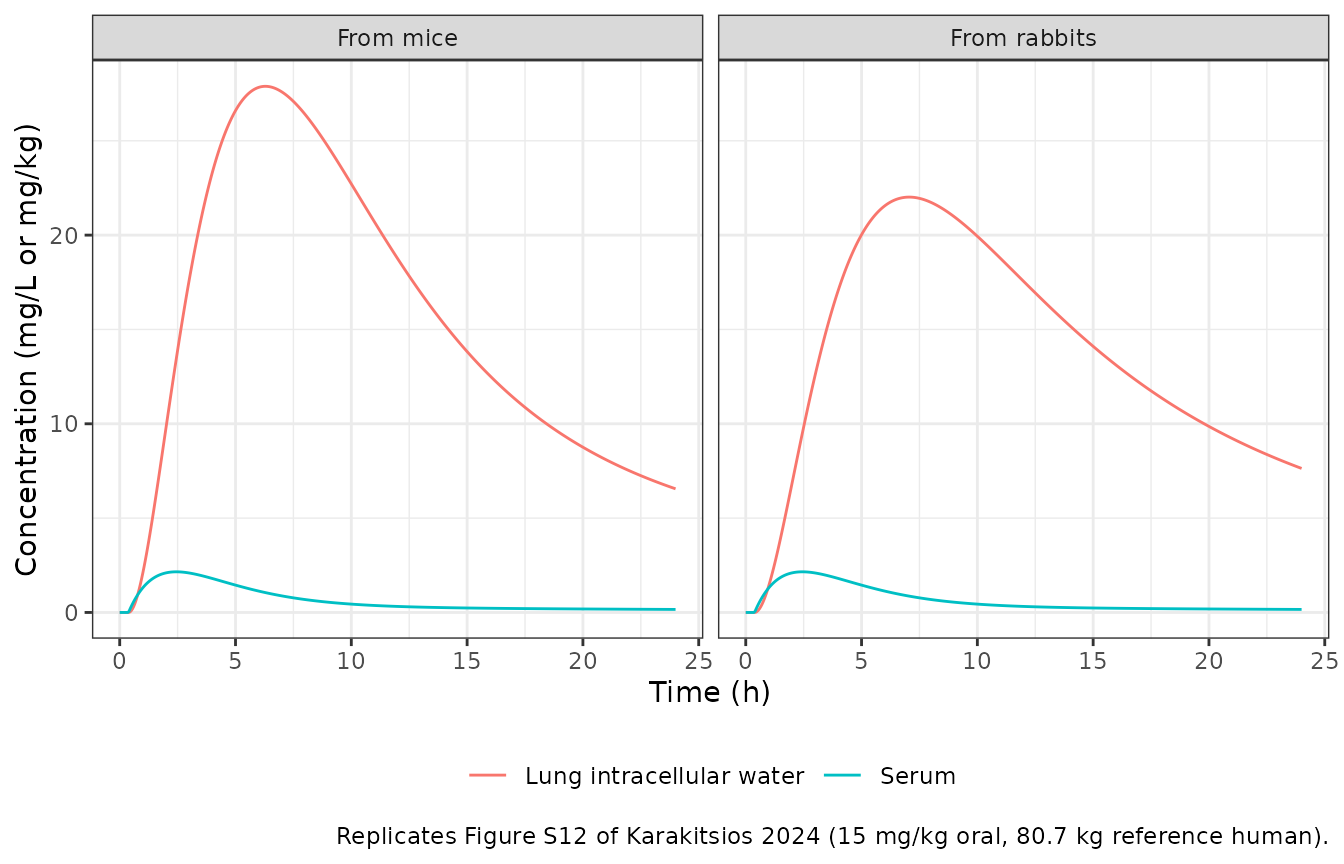
Assumptions and deviations
Rifampicin uninvolved lung does not reproduce Table 4 from
the published parameters. With the tabulated human
intracellular unbound fractions (0.058 from rabbits, 0.044 from mice;
Tables S8 and S12) and the printed equations (1)-(2), the human
uninvolved-lung AUC24 and Cmax are about 2.2-fold the Table 4
predictions and the Figure 2 PBPK curves. Every other Table 4 row,
including the rifampicin lesion and caseum rows that share the same
plasma and extracellular-water layer, reproduces within 5%, and
moxifloxacin – the other base whose lung exposure is dominated by
intracellular binding – reproduces within 5% as well. The difference is
therefore specific to how the rifampicin intracellular term was
evaluated in the authors’ implementation, which the paper does not let
us recover: matching Table 4 would need intracellular unbound fractions
of about 0.16 (rabbit-derived) and 0.11 (mouse-derived). A units slip in
the cell permeability was ruled out (scaling it 10-fold moves Tmax, not
the level). The rabbit fit shows the same pattern against Rifat 2018’s
uninvolved-lung to plasma ratio of 0.78. The published values are kept
unchanged; the rifampicin c_lung output should be read with
this in mind, while c_lesion, c_caseum and all
unbound outputs are unaffected.
Human rifampicin transit absorption. Strydom 2019 describes rifampicin absorption with a Savic transit chain but reports only ka, CL and V. Without a transit chain, AUC and Cmax match Table 4 but every Tmax is about 1.5 h early. The mean transit time was therefore back-solved from the Table 4 “Observed” Tmax of all four rifampicin tissues (1.4 h); the number of transit compartments is not identifiable (5 to 30 fit equally well) and was set to 10. Both are fixed and marked as not reported. With them, the rifampicin lesion and caseum rows also match the Table 4 PBPK predictions.
Human isoniazid clearance. Strydom 2019 estimated separate clearances for slow (9.41), intermediate (24.0) and fast (38.1 L/h) acetylators. The typical mean patient uses the cohort-weighted mean, (11 x 38.1 + 2 x 24.0 + 2 x 9.41) / 15 = 32.4 L/h, which reproduces the Table 4 “Observed” isoniazid lung exposure exactly (5.03 mg*h/kg, 0.84 mg/kg, 3 h).
Both plasma-driver choices are checked below against the Table 4
“Observed” column, which the paper obtained by simulating the Strydom
2019 empirical tissue model
dC_tissue/dt = KPL (RPL C_plasma - C_tissue) (Strydom 2019
equations 2-3, Table 3 and S3 Table). The plasma layers are taken from
the human model files themselves.
tissue_profile <- function(model, amt, kpl, rpl) {
  pl <- solve_typical(model, amt = amt)
  dt <- diff(pl$time)
  ct <- numeric(nrow(pl))
  # Exact solution of the first-order tissue equation over each 0.05 h step
  # with the plasma concentration interpolated linearly within the step.
  for (i in seq_along(dt)) {
    a <- exp(-kpl * dt[i])
    c0 <- rpl * pl$Cc[i]
    c1 <- rpl * pl$Cc[i + 1]
    slope <- (c1 - c0) / dt[i]
    ct[i + 1] <- c1 - slope / kpl + (ct[i] - c0 + slope / kpl) * a
  }
  data.frame(time = pl$time, conc = ct)
}
obs_nca <- function(d) {
  c(auc = sum(diff(d$time) * (head(d$conc, -1) + tail(d$conc, -1)) / 2),
    cmax = max(d$conc), tmax = d$time[which.max(d$conc)])
}
obs_tab <- rbind(
  "Rifampicin uninvolved lung" = obs_nca(tissue_profile(
    "Karakitsios_2024_rifampicin_human_fromRabbit_pbpk", 600, kpl = 1.68, rpl = 0.694)),
  "Isoniazid uninvolved lung" = obs_nca(tissue_profile(
    "Karakitsios_2024_isoniazid_human_fromMouse_pbpk", 300, kpl = 0.625, rpl = 0.552))
)
obs_tab <- cbind(obs_tab, "Table 4 AUC24" = c(65.56, 5.03), "Table 4 Cmax" = c(6.19, 0.84),
                 "Table 4 Tmax" = c(4.25, 3))
knitr::kable(obs_tab, digits = 2,
caption = "Strydom 2019 empirical lung model driven by this package's plasma layers.")| auc | cmax | tmax | Table 4 AUC24 | Table 4 Cmax | Table 4 Tmax | |
|---|---|---|---|---|---|---|
| Rifampicin uninvolved lung | 65.71 | 6.13 | 4.25 | 65.56 | 6.19 | 4.25 |
| Isoniazid uninvolved lung | 5.03 | 0.84 | 3.00 | 5.03 | 0.84 | 3.00 |
stopifnot(
  all(abs(obs_tab[, "auc"] / obs_tab[, "Table 4 AUC24"] - 1) < 0.02),
  all(abs(obs_tab[, "cmax"] / obs_tab[, "Table 4 Cmax"] - 1) < 0.02),
  all(abs(obs_tab[, "tmax"] - obs_tab[, "Table 4 Tmax"]) <= 0.1)
)
Moxifloxacin equations (3)-(4) are encoded in mass-conserving
form. As printed, the capillary term enters PB and EW with
signs that move drug from lower to higher unbound concentration, and PB
has no venous outflow. The files use
V_PB dC_PB/dt = Q (C_blood - C_PB) - PS_cap (fu_pls fni_pls C_PB / BP - Cu_EW fni_EW)
with the same flux entering EW. This form reproduces all three
moxifloxacin Table 4 rows within 5%.
Ionisation. The text describes the factors
W and a of equations (1)-(2) as monoprotic
Henderson-Hasselbalch terms. For these ampholytes and diprotic bases the
files use the product form, which reproduces every tabulated non-ionised
fraction (check above); W and a are applied as
full factors (unbound concentration divided by the factor = unbound
non-ionised concentration).
Rates printed as L/h. Table 3 lists the lesion and caseum distribution rates in L/h; equations (10)-(11) require 1/h, and they are used as 1/h.
Partition between PB and EW. K_EW:B is
not tabulated; it is computed as total EW over total blood concentration
when the unbound non-ionised plasma and EW concentrations are equal,
fu_pls fni_pls / (fu_EW fni_EW B/P).
Human lesion product. For humans, the product
fni_lesion x fu_lesion uses the Table S12 lesion unbound
fraction and the non-ionised fraction at the human lesion pH of 5.84.
This reproduces the rifampicin and pyrazinamide lesion rows of Table 4
within 1%.
Rabbit ethambutol plasma units. Table S10 prints clearances and volumes in mL/h and mL without a per-kg qualifier. They are read as absolute values for the 2.5 kg reference rabbit (dose 250 mg for 100 mg/kg): read per kilogram, the apparent clearance would be 23.5 L/h/kg, about twice rabbit cardiac output. Only the rabbit ethambutol file depends on this choice.
Preclinical plasma drivers. Chen 2016 models blood,
so the mouse rifampicin, ethambutol and isoniazid files feed their
central concentration to the lung directly; the Irwin 2016, Rifat 2018
and Pienaar 2017 models are plasma and are converted with the
blood-to-plasma ratio. The mouse rifampicin file uses the Chen 2016 day
1-2 clearance and the volume for doses above 1 mg/kg; the isoniazid file
keeps the Chen 2016 dose-dependent clearance through
DOSE_ISONIAZID_MGKG and the volume for doses above 0.2
mg/kg. The Rifat 2018 rifampicin infusion lasted about 10 minutes (8 mL
at 50 mL/h, Supplementary Methods). Between-animal variability of the
upstream plasma models is not carried, because the paper simulated
typical profiles; the authors’ own rabbit and human ethambutol fits keep
their Table S10 and S11 variability and residual error.
Human ethambutol dose. Figure S12 uses 15 mg/kg; this vignette applies it to the 80.7 kg reference human of Table S4. Ethambutol is not in Table 4, so there is no numeric target.