Model and source
- Citation: Wu F, Liu L, Gaudy A, Wang X, Carayannopoulos L, Pourdehnad M, Lamba M. Model based assessment of food and acid reducing agent effects on oral absorption of mezigdomide (CC-92480), a novel cereblon E3 ligase modulator. CPT Pharmacometrics Syst Pharmacol. 2023;12(10):1473-1484. doi:10.1002/psp4.13024
- Description: Two-compartment population PK model for oral mezigdomide (CC-92480), a cereblon E3 ligase modulator, in healthy subjects pooled from two phase 1 single-dose studies (Wu 2023). First-order absorption with a lag time and first-order elimination. Relative bioavailability carries high-fat-meal, proton-pump-inhibitor (rabeprazole) and formulation B effects; the absorption rate constant carries high-fat-meal and formulation-dependent PPI effects; the lag time carries a high-fat-meal effect. Inter-individual variability on CL, V1 (correlated), Q and V2; inter-occasion variability (four occasions) on ka and Tlag; combined additive plus proportional residual error.
- Article: https://doi.org/10.1002/psp4.13024 (open access; PMC10583261)
Mezigdomide (CC-92480) is an oral cereblon E3 ligase modulator in development for multiple myeloma. Wu 2023 pooled two phase 1 single-dose studies in healthy subjects to estimate the effects of a high-fat meal, of the proton-pump inhibitor (PPI) rabeprazole and of a second formulation on mezigdomide absorption. The final model (Table S2, run PK23) is a two-compartment model with first-order absorption after a lag time. Food, PPI and formulation act only on the absorption parameters (F, ka and Tlag); none of them changes clearance or the volumes.
Population
Sixty-four healthy subjects contributed 2038 plasma concentrations: 40 from Study I (NCT03803644) and 24 from Study II (NCT04211545). Mean age was 38.5 years (range 18-55), mean weight 80.1 kg (54.8-103), and 90.6% were men. By race, 56.3% were White, 40.6% Black or African American, 1.6% Asian and 1.6% American Indian or Alaska Native; 40.6% were Hispanic or Latino (Wu 2023 Table 1). Study I gave single fasted doses of 0.4, 0.8, 1.6 or 3.2 mg (part 1, six subjects per dose), then 0.8 mg fasted and after an FDA-standard high-fat meal in a two-period crossover (part 2, 16 subjects). Study II gave 1.6 mg of formulation A and of formulation B in a randomized crossover, then each formulation again after at least 7 days of rabeprazole (four periods; Figure 1).
The same information is available programmatically via
readModelDb("Wu_2023_mezigdomide")()$population.
Source trace
Every final estimate comes from Wu 2023 Figure 3a. That figure is a table printed as an image, and it reports the random effects as standard deviations (omega for IIV, gamma for IOV). The model stores variances.
| Equation / parameter | Value | Source location |
|---|---|---|
lka |
log(1.18) 1/h | Figure 3a, ka pop |
ltlag |
log(0.423) h | Figure 3a, Tlag pop |
lcl |
log(35.1) L/h | Figure 3a, CL pop |
lvc |
log(440) L | Figure 3a, V1 pop |
lq |
log(36.8) L/h | Figure 3a, Q pop |
lvp |
log(243) L | Figure 3a, V2 pop |
lfdepot |
fixed(log(1)) | Figure 3a, F pop = 1 (fixed) |
e_fed_highfat_fdepot |
0.234 | Figure 3a, beta F,FOOD |
e_form_mezigdomide_b_fdepot |
-0.236 | Figure 3a, beta F,FORMU |
e_conmed_ppi_fdepot |
-1.06 | Figure 3a, beta F,PPI |
e_fed_highfat_tlag |
1.11 | Figure 3a, beta Tlag,FOOD |
e_fed_highfat_ka |
-1.15 | Figure 3a, beta ka,FOOD |
e_conmed_ppi_forma_ka |
-0.592 | Figure 3a, beta ka,PPIA |
e_conmed_ppi_formb_ka |
-1.99 | Figure 3a, beta ka,PPIB |
etalcl, etalvc block |
0.399^2, 0.862 x 0.399 x 0.634, 0.634^2 | Figure 3a, omega CL, omega V1, corr V1,CL |
etalq |
0.262^2 | Figure 3a, omega Q |
etalvp |
0.255^2 | Figure 3a, omega V2 |
etaiov_ka_1 to _4
|
0.650^2 | Figure 3a, gamma ka; Text S1 |
etaiov_tlag_1 to _4
|
0.310^2 | Figure 3a, gamma Tlag; Text S1 |
addSd |
0.0257 ng/mL | Figure 3a, error model a |
propSd |
0.210 | Figure 3a, error model b |
| Covariate equations for log F, log ka, log Tlag; PPIA / PPIB definitions | n/a | Methods, ‘Model development and methodology’ |
d/dt(depot), d/dt(central),
d/dt(peripheral1)
|
n/a | Text S1, structural model |
Cc ~ add(addSd) + prop(propSd) + combined2() |
n/a | Text S1, y = f + e sqrt(a^2 + b^2 f^2) |
Virtual cohort
The observed data are not public. The simulation gives each of the eight dose / treatment scenarios in Figure 2 its own cohort of 150 virtual subjects. Each subject receives one single dose, so every record is on occasion 1. With one occasion per subject, the occasion-level etas on ka and Tlag act as between-subject variability, which is how the paper describes them (Text S1: they combine IIV and IOV). The model has no demographic covariates, so the cohorts need none.
scenarios <- tibble::tribble(
  ~scenario, ~dose, ~FED_HIGHFAT, ~CONMED_PPI, ~FORM_MEZIGDOMIDE_B,
  "0.4 mg, A, fasted", 0.4, 0, 0, 0,
  "0.8 mg, A, fasted", 0.8, 0, 0, 0,
  "0.8 mg, A, fed", 0.8, 1, 0, 0,
  "1.6 mg, A, fasted", 1.6, 0, 0, 0,
  "1.6 mg, B, fasted", 1.6, 0, 0, 1,
  "1.6 mg, A, fasted + PPI", 1.6, 0, 1, 0,
  "1.6 mg, B, fasted + PPI", 1.6, 0, 1, 1,
  "3.2 mg, A, fasted", 3.2, 0, 0, 0
) |>
  mutate(scenario = factor(scenario, levels = scenario))

n_per_arm <- 150L
obs_times <- c(
  0, 0.25, 0.5, 0.75, 1, 1.25, 1.5, 2, 2.5, 3, 4, 5, 6, 8, 10, 12, 16,
  24, 36, 48, 72, 96
)

make_cohort <- function(row, id_offset) {
  ids <- id_offset + seq_len(n_per_arm)
  dosing <- tibble(
    id = ids, time = 0, amt = row$dose, evid = 1L, cmt = "depot"
  )
  obs <- tidyr::expand_grid(id = ids, time = obs_times) |>
    mutate(amt = 0, evid = 0L, cmt = "central")
  bind_rows(dosing, obs) |>
    mutate(
      scenario = row$scenario,
      dose = row$dose,
      FED_HIGHFAT = row$FED_HIGHFAT,
      CONMED_PPI = row$CONMED_PPI,
      FORM_MEZIGDOMIDE_B = row$FORM_MEZIGDOMIDE_B,
      OCC = 1L
    )
}

events <- bind_rows(lapply(seq_len(nrow(scenarios)), function(i) {
  make_cohort(scenarios[i, ], id_offset = (i - 1L) * n_per_arm)
})) |>
  arrange(id, time, desc(evid))

stopifnot(!anyDuplicated(unique(events[, c("id", "time", "evid")])))
Simulation
mod <- readModelDb("Wu_2023_mezigdomide")
rxode2::rxSetSeed(20231024)
sim <- rxode2::rxSolve(
  mod,
  events = events,
  keep = c("scenario", "dose")
) |>
  as.data.frame() |>
  mutate(scenario = factor(scenario, levels = levels(scenarios$scenario)))
#> ℹ parameter labels from comments will be replaced by 'label()'
#> Warning: some etas defaulted to non-mu referenced, possible parsing error: etaiov_ka_1, etaiov_ka_2, etaiov_ka_3, etaiov_ka_4, etaiov_tlag_1, etaiov_tlag_2, etaiov_tlag_3, etaiov_tlag_4
#> as a work-around try putting the mu-referenced expression on a simple line

# Typical-value solve (no random effects) on a dense grid, one subject per
# scenario, for the closed-form AUC check below.
events_typical <- bind_rows(lapply(seq_len(nrow(scenarios)), function(i) {
  row <- scenarios[i, ]
  bind_rows(
    tibble(id = i, time = 0, amt = row$dose, evid = 1L, cmt = "depot"),
    tibble(id = i, time = seq(0, 336, by = 0.05), amt = 0, evid = 0L, cmt = "central")
  ) |>
    mutate(
      scenario = row$scenario, dose = row$dose,
      FED_HIGHFAT = row$FED_HIGHFAT, CONMED_PPI = row$CONMED_PPI,
      FORM_MEZIGDOMIDE_B = row$FORM_MEZIGDOMIDE_B, OCC = 1L
    )
}))
sim_typical <- rxode2::rxSolve(
  rxode2::zeroRe(mod),
  events = events_typical,
  keep = c("scenario", "dose")
) |>
  as.data.frame() |>
  mutate(scenario = factor(scenario, levels = levels(scenarios$scenario)))
#> ℹ parameter labels from comments will be replaced by 'label()'
#> Warning: some etas defaulted to non-mu referenced, possible parsing error: etaiov_ka_1, etaiov_ka_2, etaiov_ka_3, etaiov_ka_4, etaiov_tlag_1, etaiov_tlag_2, etaiov_tlag_3, etaiov_tlag_4
#> as a work-around try putting the mu-referenced expression on a simple line
#> Warning: some etas defaulted to non-mu referenced, possible parsing error: etaiov_ka_1, etaiov_ka_2, etaiov_ka_3, etaiov_ka_4, etaiov_tlag_1, etaiov_tlag_2, etaiov_tlag_3, etaiov_tlag_4
#> as a work-around try putting the mu-referenced expression on a simple line
#> ℹ omega/sigma items treated as zero: 'etalcl', 'etalvc', 'etalq', 'etalvp', 'etaiov_ka_1', 'etaiov_ka_2', 'etaiov_ka_3', 'etaiov_ka_4', 'etaiov_tlag_1', 'etaiov_tlag_2', 'etaiov_tlag_3', 'etaiov_tlag_4'
#> Warning: multi-subject simulation without without 'omega'
Replicate published figures
Figure 2: mean concentration-time profiles
# The pre-dose point (Cc = 0) cannot be drawn on a log axis.
sim |>
  group_by(scenario, dose, time) |>
  summarise(mean_Cc = mean(Cc), .groups = "drop") |>
  mutate(
    panel = paste(dose, "mg"),
    mean_Cc = ifelse(time == 0, NA_real_, mean_Cc)
  ) |>
  ggplot(aes(time, mean_Cc, colour = scenario)) +
  geom_line(na.rm = TRUE) +
  geom_point(size = 0.8, na.rm = TRUE) +
  geom_hline(yintercept = 0.05, linetype = "dashed", colour = "grey50") +
  facet_wrap(~panel) +
  scale_y_log10(limits = c(0.01, 10)) +
  scale_x_continuous(breaks = c(0, 24, 48, 72, 96)) +
  labs(
    x = "Time (h)", y = "Mean mezigdomide concentration (ng/mL)",
    colour = "Scenario",
    title = "Mean simulated profiles by dose and scenario",
    caption = "Replicates Figure 2 of Wu 2023. Dashed line: LLOQ 0.05 ng/mL."
  )
#> Warning in scale_y_log10(limits = c(0.01, 10)): log-10 transformation introduced infinite values.
#> log-10 transformation introduced infinite values.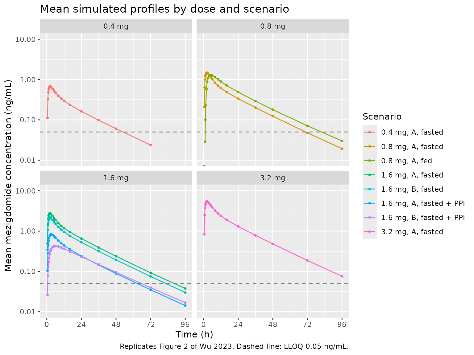
The simulated means follow the published pattern. Concentrations rise roughly in proportion to dose. After a high-fat meal the peak is later and the AUC slightly higher. Rabeprazole lowers the curve markedly with either formulation. All terminal phases run parallel, because no covariate acts on disposition.
Figure 5: visual predictive check
vpc_scen <- c(
  "0.4 mg, A, fasted", "0.8 mg, A, fasted", "0.8 mg, A, fed",
  "1.6 mg, A, fasted", "1.6 mg, A, fasted + PPI", "3.2 mg, A, fasted"
)
sim |>
  filter(scenario %in% vpc_scen) |>
  group_by(scenario, time) |>
  summarise(
    Q10 = quantile(Cc, 0.10),
    Q50 = quantile(Cc, 0.50),
    Q90 = quantile(Cc, 0.90),
    .groups = "drop"
  ) |>
  ggplot(aes(time, Q50)) +
  geom_ribbon(aes(ymin = Q10, ymax = Q90), alpha = 0.25, fill = "steelblue") +
  geom_line() +
  facet_wrap(~scenario, scales = "free_y") +
  labs(
    x = "Time (h)", y = "Mezigdomide concentration (ng/mL)",
    title = "Simulated median and 10th-90th percentiles",
    caption = paste(
      "Replicates the layout of Figure 5 of Wu 2023 (formulation A shown for",
      "the pooled 1.6 mg panels)."
    )
  )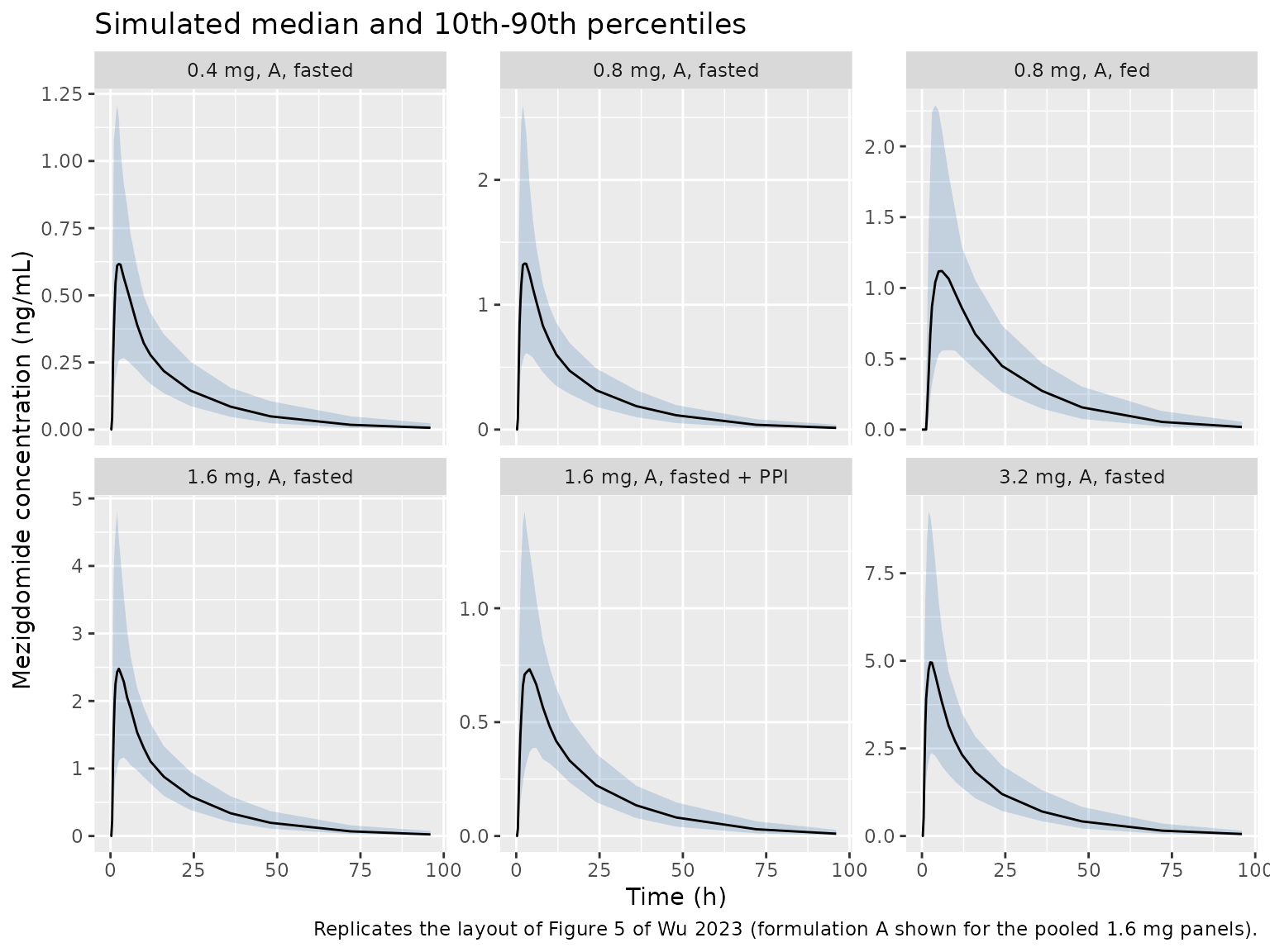
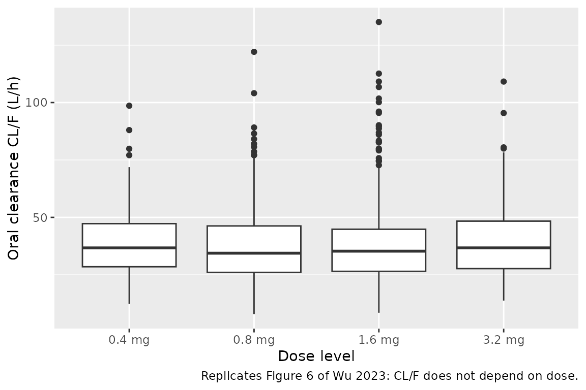
Figure 6: individual apparent clearance by dose level
sim |>
  filter(time == 0) |>
  distinct(id, dose, cl) |>
  ggplot(aes(factor(paste(dose, "mg"), levels = paste(c(0.4, 0.8, 1.6, 3.2), "mg")), cl)) +
  geom_boxplot() +
  labs(
    x = "Dose level", y = "Oral clearance CL/F (L/h)",
    caption = "Replicates Figure 6 of Wu 2023: CL/F does not depend on dose."
  )
Food, PPI and formulation effects on relative bioavailability
No covariate acts on clearance. The AUC ratio between two scenarios at the same dose therefore equals their ratio of relative bioavailability, which is exp(beta). The typical-value solve must reproduce that ratio up to numerical error, so this gate is tight.
typ_auc <- sim_typical |>
  arrange(scenario, time) |>
  group_by(scenario) |>
  summarise(
    auc = sum(diff(time) * (head(Cc, -1) + tail(Cc, -1)) / 2) +
      # Terminal extrapolation from the last two points (both in the beta phase).
      Cc[n()] / (log(Cc[n() - 1] / Cc[n()]) / (time[n()] - time[n() - 1])),
    .groups = "drop"
  )
auc_of <- function(s) typ_auc$auc[typ_auc$scenario == s]

# Exact closed form of the F ratio: AUC = F * dose / CL.
ini_vals <- rxode2::rxode(mod)$theta
#> ℹ parameter labels from comments will be replaced by 'label()'
#> Warning: some etas defaulted to non-mu referenced, possible parsing error: etaiov_ka_1, etaiov_ka_2, etaiov_ka_3, etaiov_ka_4, etaiov_tlag_1, etaiov_tlag_2, etaiov_tlag_3, etaiov_tlag_4
#> as a work-around try putting the mu-referenced expression on a simple line
f_ratio <- function(fed = 0, ppi = 0, formb = 0) {
  exp(ini_vals[["e_fed_highfat_fdepot"]] * fed +
    ini_vals[["e_conmed_ppi_fdepot"]] * ppi +
    ini_vals[["e_form_mezigdomide_b_fdepot"]] * formb)
}
typ_cl <- exp(ini_vals[["lcl"]])
auc_closed <- function(dose, ...) f_ratio(...) * dose / typ_cl * 1000

closed_check <- tibble::tribble(
  ~scenario, ~closed,
  "0.8 mg, A, fasted", auc_closed(0.8),
  "0.8 mg, A, fed", auc_closed(0.8, fed = 1),
  "1.6 mg, A, fasted", auc_closed(1.6),
  "1.6 mg, B, fasted", auc_closed(1.6, formb = 1),
  "1.6 mg, A, fasted + PPI", auc_closed(1.6, ppi = 1),
  "1.6 mg, B, fasted + PPI", auc_closed(1.6, ppi = 1, formb = 1)
) |>
  mutate(simulated = vapply(scenario, auc_of, numeric(1)))

# Trapezoidal AUC on a 0.05 h grid to 336 h with a log-linear tail; the
# remaining difference from F * dose / CL is numerical error.
stopifnot(all(abs(closed_check$simulated / closed_check$closed - 1) < 0.005))

ratios <- tibble::tribble(
  ~comparison, ~typical_sim, ~exp_beta, ~fig3b_model, ~fig3b_observed,
  "Fed / fasted (formulation A, 0.8 mg)",
  auc_of("0.8 mg, A, fed") / auc_of("0.8 mg, A, fasted"),
  f_ratio(fed = 1), 1.30, "1.29 (1.19-1.38)",
  "PPI / no PPI (formulation A, 1.6 mg)",
  auc_of("1.6 mg, A, fasted + PPI") / auc_of("1.6 mg, A, fasted"),
  f_ratio(ppi = 1), 0.360, "0.398 (0.321-0.493)",
  "PPI / no PPI (formulation B, 1.6 mg)",
  auc_of("1.6 mg, B, fasted + PPI") / auc_of("1.6 mg, B, fasted"),
  f_ratio(ppi = 1), 0.360, "0.373 (0.288-0.484)",
  "Formulation B / formulation A (1.6 mg)",
  auc_of("1.6 mg, B, fasted") / auc_of("1.6 mg, A, fasted"),
  f_ratio(formb = 1), 0.798, "0.820 (0.700-0.960)"
)

# Typical-value AUC ratio vs exp(beta): pure numerical error, so tight.
stopifnot(all(abs(ratios$typical_sim / ratios$exp_beta - 1) < 0.01))

ratios |>
  mutate(across(c(typical_sim, exp_beta), \(x) signif(x, 3))) |>
  rename(
    "Comparison" = comparison,
    "Simulated typical AUC ratio" = typical_sim,
    "exp(beta) from Figure 3a" = exp_beta,
    "Figure 3b model-predicted F ratio" = fig3b_model,
    "Figure 3b observed AUCinf ratio (90% CI)" = fig3b_observed
  ) |>
knitr::kable(caption = "AUC ratios between scenarios (Wu 2023 Figure 3b).")| Comparison | Simulated typical AUC ratio | exp(beta) from Figure 3a | Figure 3b model-predicted F ratio | Figure 3b observed AUCinf ratio (90% CI) |
|---|---|---|---|---|
| Fed / fasted (formulation A, 0.8 mg) | 1.260 | 1.260 | 1.300 | 1.29 (1.19-1.38) |
| PPI / no PPI (formulation A, 1.6 mg) | 0.346 | 0.346 | 0.360 | 0.398 (0.321-0.493) |
| PPI / no PPI (formulation B, 1.6 mg) | 0.346 | 0.346 | 0.360 | 0.373 (0.288-0.484) |
| Formulation B / formulation A (1.6 mg) | 0.790 | 0.790 | 0.798 | 0.820 (0.700-0.960) |
The packaged model gives AUC ratios equal to exp(beta) from Figure 3a: 1.26 for fed over fasted, 0.346 with rabeprazole, and 0.790 for formulation B over A. Figure 3b prints slightly different “model-predicted” ratios (1.30, 0.360, 0.798), which exp() of the Figure 3a estimates does not give. The Figure 3b caption defines its ratios as exp(beta), so they may come from another run of the model. The differences are all under 4%. Every ratio, from the Figure 3a estimates or from Figure 3b, lies inside the 90% confidence interval of the clinically observed AUCinf ratio. The largest gap between point estimates is for rabeprazole with formulation A: 0.346 from the model against 0.398 observed, 13% apart.
PKNCA validation
sim_nca <- sim |>
  filter(!is.na(Cc)) |>
  select(id, time, Cc, scenario)

sim_nca <- bind_rows(
  sim_nca,
  sim_nca |> distinct(id, scenario) |> mutate(time = 0, Cc = 0)
) |>
  distinct(id, scenario, time, .keep_all = TRUE) |>
  arrange(id, scenario, time)

dose_df <- events |>
  filter(evid == 1) |>
  select(id, time, amt, scenario)

conc_obj <- PKNCA::PKNCAconc(sim_nca, Cc ~ time | scenario + id)
dose_obj <- PKNCA::PKNCAdose(dose_df, amt ~ time | scenario + id)
intervals <- data.frame(
  start = 0, end = Inf,
  cmax = TRUE, tmax = TRUE, aucinf.obs = TRUE, half.life = TRUE
)
nca_res <- PKNCA::pk.nca(PKNCA::PKNCAdata(conc_obj, dose_obj, intervals = intervals))

nca_tab <- as.data.frame(nca_res$result) |>
  filter(PPTESTCD %in% c("cmax", "tmax", "aucinf.obs", "half.life")) |>
  group_by(scenario, PPTESTCD) |>
  summarise(median = median(PPORRES, na.rm = TRUE), .groups = "drop") |>
  tidyr::pivot_wider(names_from = PPTESTCD, values_from = median)

nca_tab |>
  mutate(across(where(is.numeric), \(x) signif(x, 3))) |>
  rename(
    "Scenario" = scenario,
    "Cmax (ng/mL)" = cmax,
    "Tmax (h)" = tmax,
    "AUCinf (ng*h/mL)" = aucinf.obs,
    "t1/2 (h)" = half.life
  ) |>
knitr::kable(caption = "Median simulated NCA parameters by scenario.")| Scenario | AUCinf (ng*h/mL) | Cmax (ng/mL) | t1/2 (h) | Tmax (h) |
|---|---|---|---|---|
| 0.4 mg, A, fasted | 10.9 | 0.634 | 16.1 | 2.5 |
| 0.8 mg, A, fasted | 24.4 | 1.360 | 15.9 | 2.5 |
| 0.8 mg, A, fed | 27.4 | 1.180 | 16.2 | 6.0 |
| 1.6 mg, A, fasted | 44.9 | 2.530 | 15.9 | 2.5 |
| 1.6 mg, B, fasted | 35.8 | 2.020 | 16.3 | 2.5 |
| 1.6 mg, A, fasted + PPI | 15.8 | 0.756 | 16.5 | 3.0 |
| 1.6 mg, B, fasted + PPI | 12.6 | 0.410 | 17.4 | 8.0 |
| 3.2 mg, A, fasted | 87.2 | 5.270 | 16.5 | 2.5 |
Wu 2023 reports no NCA table. The Results give only the observed range of Tmax: 1-4 h fasted without a PPI, and 4-8 h after the high-fat meal. The check below compares the median simulated Tmax with those ranges. The median is robust to which subjects land in the tails.
tmax_med <- setNames(nca_tab$tmax, as.character(nca_tab$scenario))
fasted_no_ppi <- c(
  "0.4 mg, A, fasted", "0.8 mg, A, fasted", "1.6 mg, A, fasted",
  "1.6 mg, B, fasted", "3.2 mg, A, fasted"
)
stopifnot(
  all(tmax_med[fasted_no_ppi] >= 1 & tmax_med[fasted_no_ppi] <= 4),
  tmax_med[["0.8 mg, A, fed"]] >= 4 & tmax_med[["0.8 mg, A, fed"]] <= 8
)
tmax_med
#>       0.4 mg, A, fasted       0.8 mg, A, fasted          0.8 mg, A, fed
#>                     2.5                     2.5                     6.0
#>       1.6 mg, A, fasted       1.6 mg, B, fasted 1.6 mg, A, fasted + PPI
#>                     2.5                     2.5                     3.0
#> 1.6 mg, B, fasted + PPI       3.2 mg, A, fasted
#>                     8.0                     2.5
Assumptions and deviations
-
Formulation labels. The Methods call formulation A
the reference (first-in-human) formulation and B the test formulation.
The Figure 1 caption swaps them. The model encodes the letter:
FORM_MEZIGDOMIDE_B = 1for formulation B and 0 for A. This matches the paper’s FORMU coding and its equations, which name the letter consistently. -
Inter-occasion variability. Monolix estimated
occasion-level random effects on ka and Tlag and no separate IIV on them
(Text S1). The model encodes this with one eta per occasion, for up to
four occasions (Study II had four periods), each with the Figure 3a
variance. Supply
OCC= 1-4 per dosing period. A record with any otherOCCgets no variability on ka or Tlag. The Discussion also lists random effects on F at the occasion level, but neither Text S1 nor Figure 3a contains such a term, so the model carries none. -
Concentration units. Doses are in mg and volumes in
L. The model multiplies by 1000 so that
Ccis in ng/mL, the unit of the assay (LLOQ 0.05 ng/mL), of Figure 2 and of the additive residual SD. -
Residual error. Text S1 gives y = f + e sqrt(a^2 +
b^2 f^2) (Monolix “combined2”). The model encodes it as
add(addSd) + prop(propSd) + combined2(). - Narrative values that differ from Figure 3a. The Discussion says the high-fat meal causes “a ~30% decrease in ka”. But exp(-1.15) = 0.32, so ka falls to about 32% of its fasted value, a 68% decrease. The model uses the Figure 3a estimate. The Figure 3b “model-predicted” F ratios also differ slightly from exp(beta); see the ratio section above.
- BLQ handling. The paper treated BLQ samples (22.5%) as left-censored. Simulations here report the full predicted concentration. The sensitivity analysis that excluded BLQ data (Table S3) is not packaged, because the paper’s final model is the censored fit in Figure 3a.
-
Screened covariates. Weight, sex, serum creatinine
and age were tested (Table S2, runs PK15-PK21) and not retained. They
are listed in
covariatesDataExcluded. - Literature check. No correction notice was found for this article (Europe PMC search, 2026-10-27).