Model and source
- Citation: Duke C, Parker SL, Zam BB, Chiong F, Sajiv C, Pawar B, Ashok A, Cooper BP, Tong SYC, Janson S, Wallis SC, Roberts JA, Tsai D. Population pharmacokinetics of unbound cefazolin in infected hospitalized patients requiring intermittent high-flux haemodialysis: can a three-times-weekly post-dialysis dosing regimen provide optimal treatment? J Antimicrob Chemother. 2024;79(11):2980-2989. doi:10.1093/jac/dkae318
- Article: https://doi.org/10.1093/jac/dkae318
- Supplement (Tables S1-S4, Figure S1): JAC Online supplementary data for the same DOI. Table S3 reproduces the final Pmetrics model file in full and is the primary transcription source for the ODE system, the covariate expression and the residual-error block.
Duke and colleagues studied the 2 g three-times-weekly post-dialysis cefazolin regimen used at their centre, in Indigenous Australian adults with end-stage kidney disease on intermittent high-flux haemodialysis. Aligning every dose with an existing dialysis session removes the need for a separate cannulation, which matters in a population that commences dialysis young and may need vascular access for decades.
This is the sibling paper of Tsai_2023_ceftriaxone, from
the same group and the same dialysis unit, and it shares that model’s
three unusual features:
-
Explicit albumin binding. Rather than assuming a
fixed unbound fraction, the model carries protein-bound cefazolin as its
own state and exchanges it with unbound drug through second-order
association (
k1) and first-order dissociation (k2) rate constants. Both total and unbound plasma concentrations are model outputs. The measured unbound fraction in this cohort (median 0.38) was roughly double the 0.21 reported for healthy volunteers. -
Dialysis replaces, rather than augments, clearance.
The Table S3 model file states
&IF (HDx.EQ.1) CL=CLHD, so while a session runs the interdialytic clearance arm is switched out entirely for a 41-fold larger dialytic clearance. This differs from the additive dialysis-arm convention used elsewhere innlmixr2lib(Veinstein_2013_gentamicin,Eyler_2014_ertapenem,Jacobs_2016_colistin,Dohmann_2025_piperacillin). -
Dialysis vintage, not creatinine, drives clearance.
Serum creatinine is uninformative in maintenance dialysis, so the
authors used the number of months since haemodialysis was started
(
T_HEMODIAL_INIT, theirTOH) as a surrogate for the progressive loss of residual renal function. Clearance falls as that time rises. The paper states this covariate had not previously been used in a popPK model for patients requiring intermittent haemodialysis.
Population
Sixteen Indigenous Australian adults (14 female, 88%) on three-times-weekly intermittent high-flux haemodialysis contributed 130 plasma samples assayed for both total and unbound cefazolin, i.e. 260 concentrations (Duke 2024 Table 1). Median age was 51 years (IQR 38.8-62.3) and median weight 69.5 kg (IQR 58.5-76.3). Median time on haemodialysis was 59 months (IQR 24.3-120) and median serum albumin 38.5 g/L (IQR 35.5-40). Median pre-dialysis urea was 19.6 mmol/L (IQR 16.2-22.8), which the Discussion invokes – together with heparin-induced free fatty acids – to explain the high unbound fraction in the absence of hypoalbuminaemia. Dialysers were high-flux throughout: FX80 (5), FX100 (10), FX120 (1). No adverse drug reactions were reported.
pop <- readModelDb("Duke_2024_cefazolin")()$population
str(pop[c("species", "n_subjects", "n_samples", "age_median", "weight_median")])
#> List of 5
#>  $ species      : chr "human"
#>  $ n_subjects   : int 16
#>  $ n_samples    : int 130
#>  $ age_median   : chr "51 years (IQR 38.8-62.3); full range not reported"
#>  $ weight_median: chr "69.5 kg (IQR 58.5-76.3); full range not reported"
Source trace
Every ini() entry carries an in-file comment naming its
source location. The table below collects them. “Table S3” refers to the
Pmetrics model file reproduced in the supplementary data.
| Equation / parameter | Value | Source location |
|---|---|---|
lcl (CLnHD) |
0.40 L/h | Table 3, Mean column (SD 0.19, CV 46.00%, median 0.39) |
lcl_hemodialysis (CLHD) |
16.36 L/h | Table 3, Mean column (SD 4.26, CV 26.04%, median 16.31) |
lvc (Vc) |
6.51 L | Table 3, Mean column (SD 1.30, CV 20.02%, median 6.74) |
lk1 (Kon) |
2.17 L/mg/h | Table 3, Mean column (SD 0.56, CV 25.86%, median 2.39) |
lk2 (Koff) |
92.13 1/h | Table 3, Mean column (SD 15.15, CV 16.44%, median 89.83) |
lk12 (Kcp) |
4.01 1/h | Table 3, Mean column (SD 2.54, CV 63.23%, median 3.51) |
lk21 (Kpc) |
1.72 1/h | Table 3, Mean column (SD 1.48, CV 86.22%, median 1.17) |
e_t_hemodial_init_cl |
0.28 (fixed) | Table S3 secondary variables: CL=CLnHD*(59/TOH)**0.28;
same form in Results |
| TOH reference 59 months | constant | Table S3 secondary variables; equals the Table 1 cohort median |
bmax_per_g_alb = 4.1 mg/g |
constant | Table S3 secondary variables: Bmax1=Alb*Vc*4.1
|
All seven eta variances |
omega^2 = log(CV^2+1) | Table 3, CV% column (see Assumptions) |
addSd, addSd_Cunbound
|
0.3 mg/L | Table S3 #Error block, C0 for both outputs |
propSd, propSd_Cunbound
|
0.1 | Table S3 #Error block, C1 for both outputs |
d/dt(central), d/dt(complex),
d/dt(peripheral1)
|
n/a | Table S3 #Differential equations (XP(1), XP(2),
XP(3)) |
Cunbound, Cc
|
n/a | Table S3 #Output equations (Y(1), Y(2)) |
| Dialysis switch | n/a | Table S3 secondary variables:
&IF (HDx.EQ.1) CL=CLHD
|
| Compartment diagram | n/a | Figure S1 |
Two independent arithmetic checks on the transcription. First, the
4.1 mg cefazolin bound per gram of albumin must reproduce
the Methods equation Bmax = Alb * N * (MCFZ / MAlb) * 1000
at 0.6 binding sites per albumin molecule, with
molecular weights of 455 and 66 500 g/mol:
0.6 * 455 / 66500 * 1000   # Table S3 rounds this to 4.1
#> [1] 4.105263
Second, Table 3’s derived half-lives carry footnote a (“Data
not available as the entry is manually calculated”), which implies they
are one-compartment hand calculations 0.693 * V / CL from
the same table’s V and CL:
c(t_half_HD  = 0.693 * 25.02 / 16.36,  # Table 3 reports 1.08 h
  t_half_nHD = 0.693 * 25.02 /  0.40,  # Table 3 reports mean 65.31 h, median 41.12
  KD_mg_L    = 92.13 / 2.17)           # Methods: KD = 1 / KA = Koff / Kon
#>  t_half_HD t_half_nHD    KD_mg_L
#>   1.059833  43.347150  42.456221
The dialysis-on half-life matches to 2%, which confirms that Table
3’s V and CLHD rows belong together as
transcribed.
Model structure
mod <- readModelDb("Duke_2024_cefazolin")
mod
#> function() {
#>   description <- "Two-compartment population PK model for intravenous cefazolin in infected Indigenous Australian adults with end-stage kidney disease on three-times-weekly intermittent high-flux haemodialysis, receiving a 2 g three-times-weekly post-dialysis regimen. PK is parameterised on unbound drug: the central state carries unbound cefazolin and an explicit second-order albumin-binding exchange (k1 on / k2 off) against a capacity bmax derived from serum albumin carries the bound drug, so total and unbound plasma concentrations are both model outputs. Clearance is replaced (not augmented) by a 41-fold higher dialytic clearance while a session is running, gated by the time-varying RRT_HEMODIAL_ACTIVE covariate; interdialytic clearance falls with the number of months the patient has been established on haemodialysis (T_HEMODIAL_INIT) through an inverse-power relationship, a surrogate for the progressive loss of residual renal function. Estimated with the Pmetrics non-parametric adaptive grid (NPAG). Duke 2024, n = 16 subjects, 130 paired total-and-unbound plasma samples."
#>   reference <- "Duke C, Parker SL, Zam BB, Chiong F, Sajiv C, Pawar B, Ashok A, Cooper BP, Tong SYC, Janson S, Wallis SC, Roberts JA, Tsai D. Population pharmacokinetics of unbound cefazolin in infected hospitalized patients requiring intermittent high-flux haemodialysis: can a three-times-weekly post-dialysis dosing regimen provide optimal treatment? J Antimicrob Chemother. 2024;79(11):2980-2989. doi:10.1093/jac/dkae318"
#>   vignette <- "Duke_2024_cefazolin"
#>   units <- list(time = "h", dosing = "mg", concentration = "mg/L")
#>
#>   # Issue #482: what each ODE state holds, in what amount units, in what
#>   # biological matrix. Mapped from the Table S3 Pmetrics model file:
#>   # X(1) = unbound drug in the central compartment, X(2) = albumin-bound
#>   # drug, X(3) = peripheral drug (Figure S1 compartment diagram).
#>   compartmentData <- list(
#>     central = list(analyte = "unbound cefazolin", units = "mg", specimen = "plasma", verified = FALSE),
#>     complex = list(analyte = "albumin-bound cefazolin", units = "mg", specimen = "plasma", verified = FALSE),
#>     peripheral1 = list(analyte = "cefazolin", units = "mg", specimen = "plasma", verified = FALSE)
#>   )
#>
#>   covariateData <- list(
#>     T_HEMODIAL_INIT = list(
#>       description = "Time the patient has been established on intermittent haemodialysis therapy for end-stage kidney disease, measured from the initiation of that therapy",
#>       units = "month",
#>       type = "continuous",
#>       reference_category = NULL,
#>       notes = "Time-fixed per subject in the source analysis. The only covariate retained in the final model (Duke 2024 Results: TOH 'was the only covariate retained in the final pharmacokinetic model'). Enters as an inverse-power effect on the interdialytic clearance arm, CL = CLnHD * (59 / TOH)^0.28 (Duke 2024 Results equation 'When dialysis is off', reproduced verbatim as 'CL=CLnHD*(59/TOH)**0.28' in the Table S3 Pmetrics model file). The 59-month reference is the cohort median TOH (Table 1: 59 months, IQR 24.3-120), so the effect is centred rather than arbitrary -- unlike the bilirubin reference in the sibling model Tsai_2023_ceftriaxone.R. Clearance and TOH followed an inverse-power relationship with r^2 = 0.433. The Discussion reads TOH as 'a surrogate for the incremental reduction in the residual renal function from the initiation of haemodialysis therapy', which is why clearance FALLS as TOH rises; the authors state this covariate had not previously been included in a popPK model for patients requiring intermittent haemodialysis. Must be strictly positive: the covariate enters as a denominator, so TOH = 0 is undefined. The paper's own dosing simulations (Table 4) span TOH = 6, 12, 24, 36 and 60 months.",
#>       source_name = "TOH"
#>     ),
#>     ALB = list(
#>       description = "Serum albumin concentration",
#>       units = "g/L",
#>       type = "continuous",
#>       reference_category = NULL,
#>       notes = "Time-fixed per subject in the source analysis. Not a covariate on any structural PK parameter; instead it sets the albumin-binding capacity of the central compartment through the Table S3 secondary variable Bmax1 = Alb * Vc * 4.1 (mg). The 4.1 mg cefazolin per g albumin constant encodes the paper's Bmax equation Bmax = Alb * N * (MCFZ / MAlb) * 1000 with N = 0.6 binding sites per albumin molecule, MCFZ = 455 g/mol and MAlb = 66500 g/mol: 0.6 * 455 / 66500 * 1000 = 4.105, rounded to 4.1 in the model file. Cohort median 38.5 g/L (IQR 35.5-40); the Discussion notes the absence of hypoalbuminaemia (< 24 g/L) in this cohort and attributes the unusually high unbound fraction to competitive displacement by uraemia (median pre-dialysis urea 19.6 mmol/L) and by heparin-induced free fatty acids instead.",
#>       source_name = "Alb"
#>     ),
#>     RRT_HEMODIAL_ACTIVE = list(
#>       description = "Haemodialysis-active indicator (1 while an intermittent high-flux haemodialysis session is running, 0 in the interdialytic interval)",
#>       units = "(binary)",
#>       type = "binary",
#>       reference_category = "0 (no dialysis session running)",
#>       notes = "Time-varying within subject. Implemented in the source as the Pmetrics conditional '&IF (HDx.EQ.1) CL=CLHD' (Table S3 secondary variables), i.e. the dialytic clearance REPLACES the interdialytic clearance arm for the duration of the session rather than being added to it. This is the opposite composition rule from the additive dialysis-arm precedents (Veinstein_2013_gentamicin.R, Eyler_2014_ertapenem.R, Jacobs_2016_colistin.R, Dohmann_2025_piperacillin.R) and follows the replacement precedent already set by the same group's Tsai_2023_ceftriaxone.R; it is encoded here as the paper wrote it. Because CLHD replaces CL entirely, the T_HEMODIAL_INIT covariate does not act during a dialysis session. Unbound cefazolin clearance was 41-fold higher during dialysis (16.36 vs 0.40 L/h), which the authors attribute to the high-flux membranes used (FX80 / FX100 / FX120, Fresenius). Doses in this study were given post-dialysis (slow push over 5 min at the completion of the session), so RRT_HEMODIAL_ACTIVE = 0 at the dosing times of the observed data. Median dialysis session duration was 4.0 h (Table 2).",
#>       source_name = "HDx"
#>     )
#>   )
#>
#>   population <- list(
#>     species = "human",
#>     n_subjects = 16L,
#>     n_studies = 1L,
#>     n_samples = 130L,
#>     age_median = "51 years (IQR 38.8-62.3); full range not reported",
#>     weight_median = "69.5 kg (IQR 58.5-76.3); full range not reported",
#>     sex_female_pct = 87.5,
#>     race_ethnicity = "100% Indigenous Australian (an explicit inclusion criterion). The Discussion notes that this population commences haemodialysis considerably younger than their non-Indigenous counterparts, which is why vein preservation -- and therefore a post-dialysis regimen requiring no separate cannulation -- carries particular weight.",
#>     disease_state = "Adults with end-stage kidney disease established on three-times-weekly intermittent high-flux haemodialysis, treated with cefazolin for an active infection or for surgical prophylaxis. Indications as printed in Table 1: line-associated cellulitis (4), wound infection (3), abscess (3), bacteraemia (3), diabetic foot infection (2), periorbital cellulitis (2), surgical prophylaxis (1). Baseline laboratory values (median, IQR): albumin 38.5 g/L (35.5-40), pre-dialysis urea 19.6 mmol/L (16.2-22.8), total bilirubin 7.5 umol/L (6-12), ALP 233 U/L (179-307), GGT 142 U/L (71-192), ALT 9 U/L (5.75-18.75). No adverse drug reactions were reported.",
#>     renal_function = "End-stage kidney disease requiring three-times-weekly intermittent haemodialysis. Residual renal function could not be quantified because serum creatinine in maintenance-dialysis patients is dominated by time since the last session (stated study limitation); the authors used months since initiation of haemodialysis (TOH, median 59, IQR 24.3-120) as its surrogate instead. Dialysers were high-flux throughout: FX80 in 5 subjects, FX100 in 10, FX120 in 1 (ultrafiltration coefficients 59, 73 and 87 mL/h/mmHg; surface areas 1.8, 2.2 and 2.5 m^2). Dialysis parameters (Table S4, mean +/- SD): blood flow rate 348 +/- 47 mL/min, ultrafiltration volume 2939 +/- 819 mL, Kt/V 1.69 +/- 0.37, recirculation 11.4 +/- 1.9%. No subject received haemodiafiltration.",
#>     dose_range = "2 g cefazolin (Cefazolin-AFT) reconstituted in 10 mL water-for-injection and injected through the arteriovenous fistula or central line as a slow push over 5 min at the completion of each dialysis session, three times weekly.",
#>     regions = "Australia (renal dialysis unit of a remote Northern Territory hospital, Alice Springs)",
#>     protein_binding = "Measured directly rather than assumed: median unbound fraction 0.38 (IQR 0.32-0.46), roughly double the 0.21 reported for healthy volunteers. Median pre-dialysis unbound trough was 35.7 mg/L (IQR 27.5-45.7) over a 2-day interval and 17.7 mg/L (IQR 13.5-31.4) over a 3-day interval; the lowest pre-dialysis unbound concentration observed in the whole study was 9.1 mg/L. The unbound fraction was higher immediately before dialysis than immediately after (mean 36.5% +/- 6.8% versus 24.5% +/- 14.3%).",
#>     notes = "Prospective single-centre population PK study. 260 concentrations (130 total, 130 unbound) from 16 patients. Plasma sampled over two dosing or dialysis intervals: directly before dialysis, immediately after dialysis, then 5, 15, 60 and 1440 min after the dose, then at 48 h or immediately before the next dialysis session (whichever came first), and again before the next session when the interval was 72 h. Total and unbound cefazolin assayed 1-500 mg/L by validated UHPLC-MS/MS (Table S1); the unbound fraction was isolated by ultrafiltration at 37 C with Centrifree devices. Exclusion criteria: pregnancy, cephalosporin allergy, or a requirement for more frequent dialysis."
#>   )
#>
#>   ini({
#>     # Structural parameters: Duke 2024 Table 3, 'Mean' column of the
#>     # Pmetrics NPAG non-parametric population distribution. Table 3 also
#>     # reports a 'Median' column; the mean is used as the typical value
#>     # here (it is the column the Abstract, Results and Discussion quote)
#>     # and the median is noted per line. Only the seven primary variables
#>     # of the Table S3 model file are estimated; V and the two half-lives
#>     # in Table 3 carry footnote 'a' ("Data not available as the entry is
#>     # manually calculated") and are derived quantities, not model
#>     # parameters.
#>     lcl <- log(0.40)
#>     label("Interdialytic (dialysis-off) clearance CLnHD (L/h)")
#>     # Duke 2024 Table 3: CLnHD mean 0.40, SD 0.19, CV 46.00%, median 0.39 L/h
#>
#>     lcl_hemodialysis <- log(16.36)
#>     label("Intradialytic (dialysis-on) clearance CLHD (L/h)")
#>     # Duke 2024 Table 3: CLHD mean 16.36, SD 4.26, CV 26.04%, median 16.31 L/h
#>
#>     lvc <- log(6.51)
#>     label("Central volume of distribution Vc (L)")
#>     # Duke 2024 Table 3: Vc mean 6.51, SD 1.30, CV 20.02%, median 6.74 L
#>
#>     lk1 <- log(2.17)
#>     label("Second-order cefazolin-albumin association rate constant Kon (L/mg/h)")
#>     # Duke 2024 Table 3: Kon mean 2.17, SD 0.56, CV 25.86%, median 2.39 L/mg/h
#>
#>     lk2 <- log(92.13)
#>     label("First-order cefazolin-albumin dissociation rate constant Koff (1/h)")
#>     # Duke 2024 Table 3: Koff mean 92.13, SD 15.15, CV 16.44%, median 89.83 1/h
#>     # Implied KD = Koff / Kon = 92.13 / 2.17 = 42.46 mg/L (Methods: KD = 1/KA = Koff/Kon)
#>
#>     lk12 <- log(4.01)
#>     label("Central-to-peripheral rate constant Kcp (1/h)")
#>     # Duke 2024 Table 3: Kcp mean 4.01, SD 2.54, CV 63.23%, median 3.51 1/h
#>
#>     lk21 <- log(1.72)
#>     label("Peripheral-to-central rate constant Kpc (1/h)")
#>     # Duke 2024 Table 3: Kpc mean 1.72, SD 1.48, CV 86.22%, median 1.17 1/h
#>
#>     # Time-on-haemodialysis effect on the interdialytic clearance arm. The
#>     # exponent is hard-coded in the Table S3 model file rather than
#>     # reported as an estimated parameter in Table 3, so it is encoded as
#>     # fixed().
#>     e_t_hemodial_init_cl <- fixed(0.28)
#>     label("Inverse-power exponent of months on haemodialysis on interdialytic CL (unitless)")
#>     # Duke 2024 Table S3 secondary variables: CL=CLnHD*(59/TOH)**0.28;
#>     # same form printed in Results ('When dialysis is off'). Equivalent to
#>     # (TOH / 59)^-0.28. Supported by the reported inverse-power fit,
#>     # r^2 = 0.433.
#>
#>     # Interindividual variability. Pmetrics NPAG estimates a discrete
#>     # non-parametric distribution rather than a parametric omega matrix;
#>     # Table 3 summarises that distribution by its mean, SD and CV%. The
#>     # CV% is carried here into a log-normal random effect using the
#>     # standard omega^2 = log(CV^2 + 1) identity. This is a parametric
#>     # APPROXIMATION of a non-parametric distribution (see vignette
#>     # 'Assumptions and deviations'); it is required to reproduce the
#>     # paper's own Monte Carlo PTA simulations, which sample the
#>     # population distribution.
#>     #   CLnHD : 46.00% CV -> omega^2 = log(0.4600^2 + 1) = 0.191942
#>     #   CLHD  : 26.04% CV -> omega^2 = log(0.2604^2 + 1) = 0.065608
#>     #   Vc    : 20.02% CV -> omega^2 = log(0.2002^2 + 1) = 0.039298
#>     #   Kon   : 25.86% CV -> omega^2 = log(0.2586^2 + 1) = 0.064733
#>     #   Koff  : 16.44% CV -> omega^2 = log(0.1644^2 + 1) = 0.026669
#>     #   Kcp   : 63.23% CV -> omega^2 = log(0.6323^2 + 1) = 0.336332
#>     #   Kpc   : 86.22% CV -> omega^2 = log(0.8622^2 + 1) = 0.555831
#>     etalcl              ~ 0.191942  # Duke 2024 Table 3 (CLnHD, CV 46.00%)
#>     etalcl_hemodialysis ~ 0.065608  # Duke 2024 Table 3 (CLHD,  CV 26.04%)
#>     etalvc              ~ 0.039298  # Duke 2024 Table 3 (Vc,    CV 20.02%)
#>     etalk1              ~ 0.064733  # Duke 2024 Table 3 (Kon,   CV 25.86%)
#>     etalk2              ~ 0.026669  # Duke 2024 Table 3 (Koff,  CV 16.44%)
#>     etalk12             ~ 0.336332  # Duke 2024 Table 3 (Kcp,   CV 63.23%)
#>     etalk21             ~ 0.555831  # Duke 2024 Table 3 (Kpc,   CV 86.22%)
#>
#>     # Residual error. Table S3 '#Error' block gives one assay-error
#>     # polynomial per output equation, identical for both:
#>     #   0.3, 0.1, 0, 0   ->  SD = 0.3 + 0.1 * conc  (C2 = C3 = 0)
#>     # so each output carries a 0.3 mg/L additive plus 10% proportional
#>     # term. The C1 = 0.1 slope is consistent with the Table S1 assay
#>     # validation (total-cefazolin precision 4.1-5.3%, unbound 3.6-6.3%).
#>     # NOTE: Pmetrics multiplies this assay polynomial by an estimated
#>     # noise-inflation factor gamma; the Table S3 file sets the gamma
#>     # STARTING value 'G=2', and the paper does not report the final
#>     # estimated gamma anywhere. The assay polynomial is therefore carried
#>     # here unscaled (equivalent to gamma = 1), which is the minimum-
#>     # assumption reading of the Table S3 file, matching the sibling
#>     # extraction Tsai_2023_ceftriaxone.R. See vignette 'Assumptions and
#>     # deviations'.
#>     addSd <- 0.3
#>     label("Additive residual error on total Cc (mg/L)")
#>     # Duke 2024 Table S3 #Error, output 2 (total): C0 = 0.3
#>     propSd <- 0.1
#>     label("Proportional residual error on total Cc (fraction)")
#>     # Duke 2024 Table S3 #Error, output 2 (total): C1 = 0.1
#>     addSd_Cunbound <- 0.3
#>     label("Additive residual error on unbound Cunbound (mg/L)")
#>     # Duke 2024 Table S3 #Error, output 1 (unbound): C0 = 0.3
#>     propSd_Cunbound <- 0.1
#>     label("Proportional residual error on unbound Cunbound (fraction)")
#>     # Duke 2024 Table S3 #Error, output 1 (unbound): C1 = 0.1
#>   })
#>
#>   model({
#>     # Stoichiometric constant for the albumin-binding capacity, carried
#>     # exactly as hard-coded in the Table S3 secondary variable
#>     # Bmax1 = Alb * Vc * 4.1. Units: mg cefazolin bound per g albumin.
#>     # It encodes the Methods equation Bmax = Alb * N * (MCFZ/MAlb) * 1000
#>     # with N = 0.6 binding sites per albumin molecule --
#>     #   0.6 * 455 (cefazolin g/mol) / 66500 (albumin g/mol) * 1000 = 4.105
#>     # -- which the model file rounds to 4.1.
#>     bmax_per_g_alb <- 4.1
#>
#>     # Reference time on haemodialysis for the inverse-power clearance
#>     # covariate (months). Hard-coded in the Table S3 model file; it is the
#>     # Table 1 cohort median TOH of 59 months.
#>     toh_ref <- 59
#>
#>     # Individual parameters.
#>     cl              <- exp(lcl + etalcl) * (toh_ref / T_HEMODIAL_INIT)^e_t_hemodial_init_cl
#>     cl_hemodialysis <- exp(lcl_hemodialysis + etalcl_hemodialysis)
#>     vc              <- exp(lvc + etalvc)
#>     k1              <- exp(lk1 + etalk1)
#>     k2              <- exp(lk2 + etalk2)
#>     k12             <- exp(lk12 + etalk12)
#>     k21             <- exp(lk21 + etalk21)
#>
#>     # Dialysis REPLACES the interdialytic clearance arm rather than adding
#>     # to it (Table S3: '&IF (HDx.EQ.1) CL=CLHD'). Note this differs from
#>     # the additive dialysis-arm convention used by Veinstein 2013 /
#>     # Eyler 2014 / Jacobs 2016 / Dohmann 2025; it follows the same group's
#>     # Tsai 2023 ceftriaxone model and is encoded as Duke 2024 wrote it.
#>     cl_total <- (1 - RRT_HEMODIAL_ACTIVE) * cl + RRT_HEMODIAL_ACTIVE * cl_hemodialysis
#>     kel      <- cl_total / vc
#>
#>     # Albumin-binding capacity of the central compartment, as a MASS (mg)
#>     # rather than a concentration -- so it is directly comparable with the
#>     # bound-drug amount held in the 'complex' state (Table S3 Bmax1).
#>     bmax <- ALB * vc * bmax_per_g_alb
#>
#>     # ODE system, transcribed from the Table S3 '#Differential equations'
#>     # block. X(1) -> central (unbound drug), X(2) -> complex (albumin-bound
#>     # drug), X(3) -> peripheral1. Elimination and inter-compartmental
#>     # distribution act on unbound drug only; the bound state exchanges
#>     # solely with central.
#>     #   XP(1) = RATEIV(1) - (Ke + Kcp)*X(1) - (Kon/Vc)*(Bmax1-X(2))*X(1)
#>     #                     + Koff*X(2) + Kpc*X(3)
#>     #   XP(2) =             (Kon/Vc)*(Bmax1-X(2))*X(1) - Koff*X(2)
#>     #   XP(3) =  Kcp*X(1) - Kpc*X(3)
#>     # The dose enters 'central' (Pmetrics RATEIV(1)) via the event table.
#>     # At binding equilibrium this system reproduces the paper's Methods
#>     # relation Ctotal = Cunbound + Bmax * Cunbound / (KD + Cunbound) with
#>     # KD = Koff / Kon and Bmax = Alb * 4.1 mg/L.
#>     d/dt(central) <- -(kel + k12) * central -
#>       (k1 / vc) * (bmax - complex) * central + k2 * complex + k21 * peripheral1
#>     d/dt(complex) <-
#>       (k1 / vc) * (bmax - complex) * central - k2 * complex
#>     d/dt(peripheral1) <- k12 * central - k21 * peripheral1
#>
#>     # Output equations (Table S3 '#Output equations').
#>     #   Y(1) = X(1)/Vc          -> unbound plasma concentration
#>     #   Y(2) = (X(2)+X(1))/Vc   -> total plasma concentration
#>     Cunbound <- central / vc
#>     Cc       <- (complex + central) / vc
#>
#>     Cc       ~ add(addSd) + prop(propSd)
#>     Cunbound ~ add(addSd_Cunbound) + prop(propSd_Cunbound)
#>   })
#> }
#> <environment: 0x5613dc030b58>
Virtual cohort
Original observed data are not publicly available. The cohort below reproduces the Table 1 covariate distributions: time on haemodialysis log-normal with median 59 months and an IQR close to the observed 24.3-120, and serum albumin centred on the observed median of 38.5 g/L.
set.seed(20241110)
n_sub <- 200L  # 200 per arm is the vignette cap

cohort <- tibble(
  id              = seq_len(n_sub),
  T_HEMODIAL_INIT = pmax(1, rlnorm(n_sub, meanlog = log(59), sdlog = 1.18)),
  ALB             = pmax(20, rnorm(n_sub, mean = 38.5, sd = 3.4))
)

quantile(cohort$T_HEMODIAL_INIT, c(0.25, 0.5, 0.75))  # paper: 59 (IQR 24.3-120) months
#>       25%       50%       75%
#>  24.44566  53.57493 131.37807
quantile(cohort$ALB,             c(0.25, 0.5, 0.75))  # paper: 38.5 (IQR 35.5-40) g/L
#>      25%      50%      75%
#> 35.92423 38.10502 40.81433
A helper builds event tables. Three points matter:
- This model declares two endpoints (
CcandCunbound), each with its own residual-error term, and neither is an ODE state – both are algebraic observables built fromcentral,complexandperipheral1. rxode2 injects a compartment slot for each endpoint after the ODE states and then requires thedvid->cmtmap to be satisfied, so observation rows carrycmt = NA_character_plus an explicitdvid = 1L. Pointingcmtat an ODE state (cmt = "central") on an observation row fails with'dvid'->'cmt' ... undefined compartment.dvidis set on the dose rows too so the column is notNA-typed. Both observables come back as columns regardless of which endpointdvidnames. -
RRT_HEMODIAL_ACTIVEis genuinely time-varying, so the event table is built as a plain data frame and the covariate column is set per row. Assigning covariates onto anrxEtobject instead would silently drop them. - Each dose is given as a 5 min infusion
(
dur), matching the paper’s “slow push over 5 min” and theRATEIV(1)input of the Table S3 model file. A bolus would put the entire dose intocentralas unbound drug att = 0, before any binding has occurred, producing a spurious unbound spike.
SESSION_H  <- 4.0     # Table 2: median dialysis session duration 4.0 h
PUSH_H     <- 5 / 60  # Methods: slow push over 5 min

make_events <- function(subjects, dose_mg, dose_times, obs_times,
                        sessions = NULL, id_offset = 0L, label = NA_character_) {
  rows <- lapply(seq_len(nrow(subjects)), function(i) {
    sid <- id_offset + subjects$id[i]
    dose_rows <- data.frame(
      id = sid, time = dose_times, amt = dose_mg, evid = 1L,
      dur = PUSH_H, cmt = "central", dvid = 1L
    )
    obs_rows <- data.frame(
      id = sid, time = obs_times, amt = 0, evid = 0L,
      dur = NA_real_, cmt = NA_character_, dvid = 1L
    )
    ev <- dplyr::arrange(dplyr::bind_rows(dose_rows, obs_rows), time, dplyr::desc(evid))
    ev$T_HEMODIAL_INIT <- subjects$T_HEMODIAL_INIT[i]
    ev$ALB             <- subjects$ALB[i]
    ev$treatment       <- label
    on <- rep(FALSE, nrow(ev))
    for (s in sessions) on <- on | (ev$time >= s[1] & ev$time < s[2])
    ev$RRT_HEMODIAL_ACTIVE <- as.numeric(on)
    ev
  })
  dplyr::bind_rows(rows)
}
The paper’s simulations assume dialysis on Days 1, 4 and 6, so sessions start 72, 48 and 48 h apart and each dose is given at the end of its session. That schedule is used for every steady-state result below.
WEEK_H     <- 168
sess_start <- sort(as.vector(outer(c(0, 72, 120), seq(0, 4) * WEEK_H, "+")))
sessions   <- lapply(sess_start, function(s) c(s, s + SESSION_H))
dose_times <- sess_start + SESSION_H

# Session starts bounding the fourth simulated week. A pre-dialysis trough is
# the value immediately before one of these. Every element must itself be a
# session start, or the "reduction across a session" below would silently
# measure an interval in which no dialysis ran.
week4 <- c(504, 576, 624, 672)
eps   <- 1e-6
stopifnot(all(week4 %in% sess_start))

# Interval lengths preceding each: 72 h then 48 h then 48 h, i.e. Days 1, 4, 6.
diff(week4)
#> [1] 72 48 48
Simulation
rxSolve() redraws the random effects on every call, so
each scenario below is preceded by rxSetSeed() with the
same value. That gives the arms common random numbers:
differences between them are then attributable to dose and covariate,
not to two independent draws of a 200-subject cohort.
obs_ss <- sort(unique(c(
  seq(0, 504, by = 4),                       # burn-in to steady state, coarse
  seq(504, 680, by = 0.5),                   # final week, fine
  dose_times, sess_start, sess_start + SESSION_H,
  week4 - eps, week4 + SESSION_H - eps
)))

ev_ss <- make_events(cohort, dose_mg = 2000, dose_times = dose_times,
                     obs_times = obs_ss, sessions = sessions,
                     label = "2 g three times weekly")

rxode2::rxSetSeed(20241110)
sim_ss <- rxode2::rxSolve(mod, events = ev_ss, sigma = NA,
                          keep = c("T_HEMODIAL_INIT", "ALB", "RRT_HEMODIAL_ACTIVE")) |>
  as.data.frame()
#> ℹ parameter labels from comments will be replaced by 'label()'

at <- function(tt) dplyr::arrange(dplyr::filter(sim_ss, abs(time - tt) < 1e-9), id)
nrow(sim_ss)
#> [1] 98200
Typical-value profiles use omega = NA rather than
zeroRe(), because zeroRe() mutates shared
model state.
typ <- tibble(id = 1L, T_HEMODIAL_INIT = 59, ALB = 38.5) # cohort mediansReplicate published figures
Figure 1 – total and unbound concentration-time profiles
Figure 1 of Duke 2024 shows observed total (grey) and unbound (black) cefazolin with the final model’s predicted lines for each patient. Here the typical-value profile is shown across a full weekly cycle, which exposes both the slow interdialytic decline and the sharp intradialytic drops.
wk_sess  <- Filter(function(s) s[1] >= 504 && s[1] <= 672, sessions)
wk_dose  <- dose_times[dose_times >= 504 & dose_times < 672]
wk_obs   <- sort(unique(c(seq(0, 680, by = 1), seq(504, 680, by = 0.25),
                          dose_times, sess_start, sess_start + SESSION_H)))

rxode2::rxSetSeed(20241110)
ev_typ  <- make_events(typ, dose_mg = 2000, dose_times = dose_times,
                       obs_times = wk_obs, sessions = sessions, label = "typical")
sim_typ <- rxode2::rxSolve(mod, events = ev_typ, omega = NA, sigma = NA) |>
  as.data.frame() |>
  filter(time >= 500, time <= 676)

sess_df <- do.call(rbind, lapply(wk_sess, function(s) data.frame(xmin = s[1], xmax = s[2])))

sim_typ |>
  select(time, Total = Cc, Unbound = Cunbound) |>
  pivot_longer(-time, names_to = "Analyte", values_to = "conc") |>
  ggplot(aes(time - 504, conc, colour = Analyte)) +
  geom_rect(data = sess_df, inherit.aes = FALSE,
            aes(xmin = xmin - 504, xmax = xmax - 504, ymin = 1, ymax = Inf),
            fill = "grey70", alpha = 0.4) +
  geom_line(linewidth = 0.7) +
  scale_y_log10() +
  scale_colour_manual(values = c(Total = "grey40", Unbound = "black")) +
  labs(x = "Time within the weekly cycle (h)", y = "Cefazolin concentration (mg/L)",
       title = "Steady-state weekly cycle, 2 g three times weekly post-dialysis",
       caption = "Replicates the structure of Figure 1 of Duke 2024.")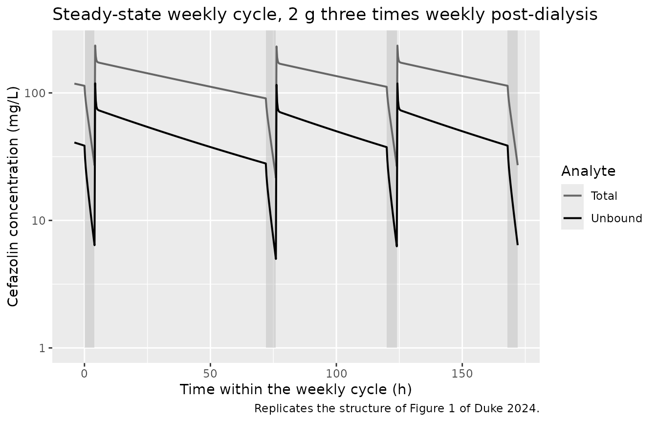
Replicates the structure of Figure 1 of Duke 2024: typical-value total and unbound cefazolin across one weekly cycle of the 2 g three-times-weekly post-dialysis regimen. Shaded bands are dialysis sessions.
Clearance versus time on haemodialysis
The paper reports an inverse-power relationship between unbound cefazolin clearance and months on haemodialysis (r^2 = 0.433), reproduced from the Table S3 expression.
tibble(TOH = seq(1, 180, by = 0.5)) |>
  mutate(CL = 0.40 * (59 / TOH)^0.28) |>
  ggplot(aes(TOH, CL)) +
  geom_line(linewidth = 0.8) +
  geom_vline(xintercept = 59, linetype = "dashed", colour = "grey50") +
  annotate("text", x = 59, y = 0.95, label = "reference 59 months",
           hjust = -0.05, size = 3, colour = "grey30") +
  labs(x = "Time on haemodialysis (months)",
       y = "Interdialytic clearance CL (L/h)",
       title = "CL = CLnHD * (59 / TOH)^0.28",
       caption = "Duke 2024 reports an inverse-power fit with r^2 = 0.433.")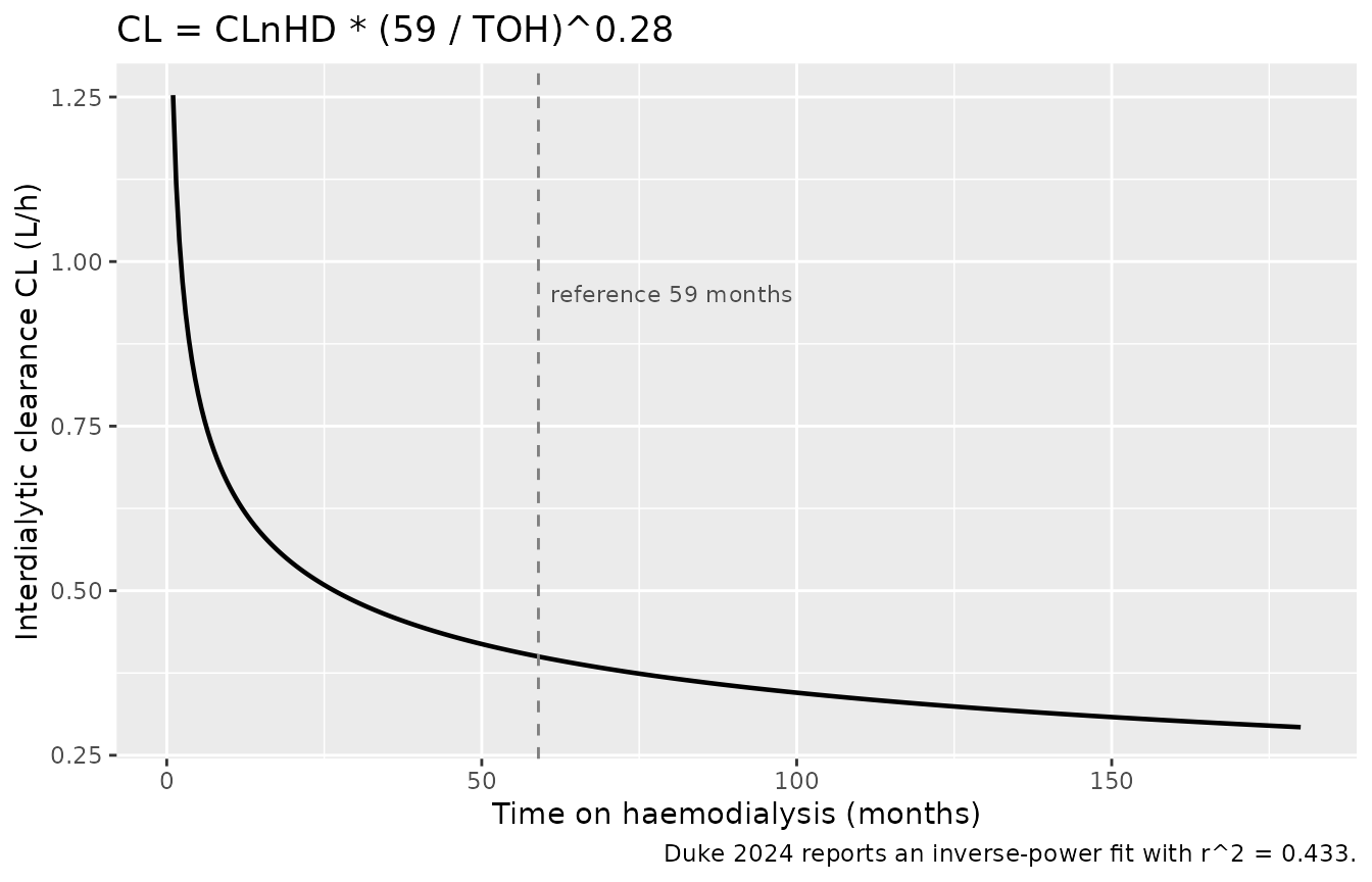
The inverse-power relationship between interdialytic unbound cefazolin clearance and time on haemodialysis (Duke 2024 Results, ‘When dialysis is off’).
Protein binding
The paper reports a median unbound fraction of 0.38 (IQR 0.32-0.46), roughly double the 0.21 typical of healthy volunteers. The explicit binding model reproduces this without any fitted unbound-fraction parameter.
fu_df <- sim_ss |>
  filter(time > 504, !is.na(Cc), Cc > 1) |>
  mutate(fu = Cunbound / Cc)

tibble(
  Source = c("Simulated", "Duke 2024 (observed)"),
  Q1     = c(quantile(fu_df$fu, 0.25), 0.32),
  Median = c(median(fu_df$fu),         0.38),
  Q3     = c(quantile(fu_df$fu, 0.75), 0.46)
) |>
  rename("Unbound fraction" = Source) |>
knitr::kable(digits = 3, caption = "Unbound fraction: simulated vs Duke 2024 Table 2.")| Unbound fraction | Q1 | Median | Q3 |
|---|---|---|---|
| Simulated | 0.307 | 0.353 | 0.401 |
| Duke 2024 (observed) | 0.320 | 0.380 | 0.460 |
ggplot(fu_df, aes(fu)) +
  geom_histogram(bins = 50, fill = "grey60", colour = "white") +
  geom_vline(xintercept = c(0.32, 0.38, 0.46), linetype = c(3, 1, 3)) +
  labs(x = "Unbound fraction", y = "Count",
       title = "Simulated unbound fraction at steady state",
       caption = "Solid line = Duke 2024 median 0.38; dotted = reported IQR 0.32-0.46.")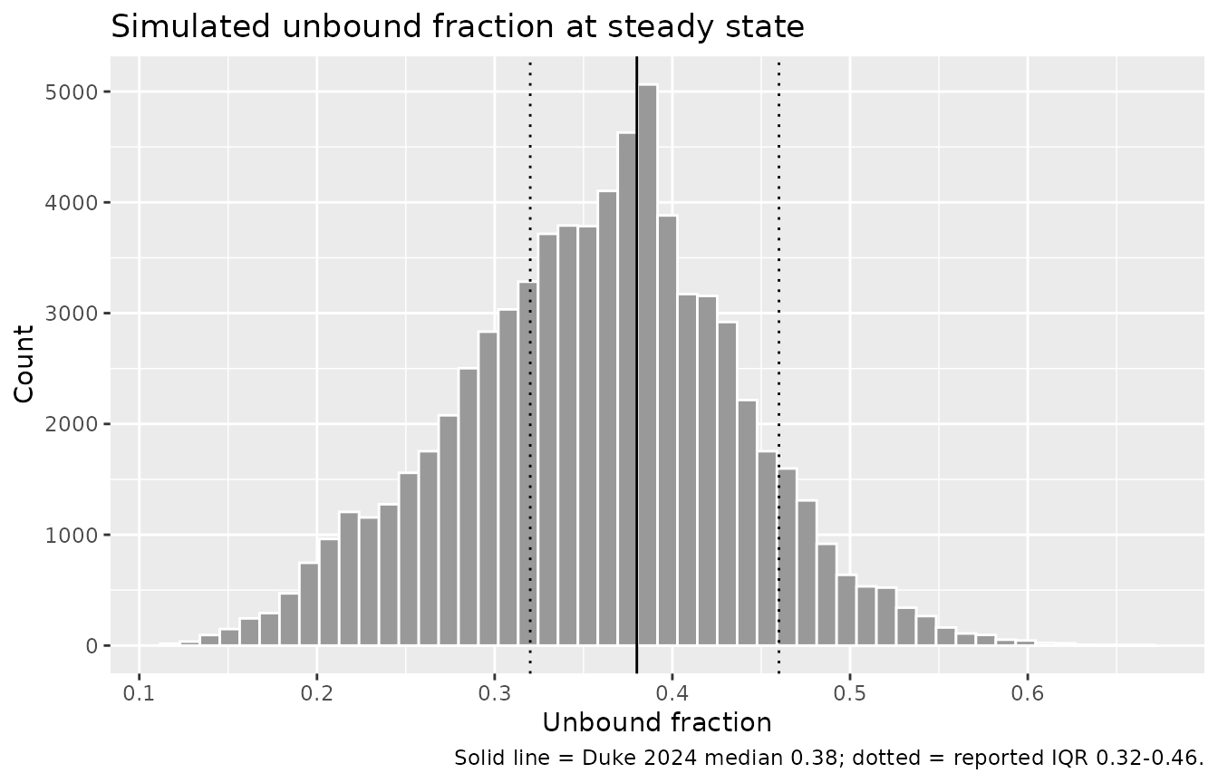
Simulated unbound fraction at steady state versus the values reported by Duke 2024.
The binding is saturable, so the unbound fraction is concentration
dependent: at the equilibrium of the two binding fluxes the model
reduces exactly to the paper’s Methods relation
Ctotal = Cunbound + Bmax * Cunbound / (KD + Cunbound).
KD   <- 92.13 / 2.17                 # mg/L
Bmax <- 38.5 * 4.1                   # mg/L at the median albumin of 38.5 g/L
cu   <- c(2, 10, 17.7, 35.7, 100)
data.frame(
  Cunbound = cu,
  Ctotal   = cu + Bmax * cu / (KD + cu),
  fu       = cu / (cu + Bmax * cu / (KD + cu))
)
#>   Cunbound     Ctotal        fu
#> 1      2.0   9.101368 0.2197472
#> 2     10.0  40.091760 0.2494278
#> 3     17.7  64.144822 0.2759381
#> 4     35.7 107.802322 0.3311617
#> 5    100.0 210.805972 0.4743699
Dialysis effect
Two reported quantities probe the dialysis switch: clearance is 41-fold higher during a session, and concentrations fall sharply across each session (Table 2: total by a median 72.6%, unbound by 83.3%).
c(CLnHD = 0.40, CLHD = 16.36, ratio = 16.36 / 0.40)
#> CLnHD  CLHD ratio
#>  0.40 16.36 40.90

reduction <- bind_rows(lapply(week4, function(st) {
  pre  <- at(st - eps)
  post <- at(st + SESSION_H - eps)   # just BEFORE the post-dialysis dose
  data.frame(id      = pre$id,
             unbound = 100 * (1 - post$Cunbound / pre$Cunbound),
             total   = 100 * (1 - post$Cc       / pre$Cc))
}))

tibble(
  Analyte = c("Unbound", "Unbound", "Total", "Total"),
  Source  = c("Simulated", "Duke 2024", "Simulated", "Duke 2024"),
  Q1      = c(quantile(reduction$unbound, 0.25), 78.7, quantile(reduction$total, 0.25), 69.2),
  Median  = c(median(reduction$unbound),         83.3, median(reduction$total),         72.6),
  Q3      = c(quantile(reduction$unbound, 0.75), 86.3, quantile(reduction$total, 0.75), 75.8)
) |>
  knitr::kable(digits = 1, caption = paste(
    "Concentration reduction across one 4.0 h dialysis session,",
    "simulated vs Duke 2024 Table 2."
))| Analyte | Source | Q1 | Median | Q3 |
|---|---|---|---|---|
| Unbound | Simulated | 72.4 | 81.0 | 89.4 |
| Unbound | Duke 2024 | 78.7 | 83.3 | 86.3 |
| Total | Simulated | 63.8 | 72.9 | 85.0 |
| Total | Duke 2024 | 69.2 | 72.6 | 75.8 |
# Structural: the median per-session unbound reduction must land near the
# reported 83.3%. A mis-transcribed CLHD or a mis-gated dialysis switch moves
# this by tens of percentage points. Asserted on the MEDIAN, not on any subject
# extreme, so the bound is stable across rxode2 random draws.
stopifnot(abs(median(reduction$unbound) - 83.3) < 8,
          abs(median(reduction$total)   - 72.6) < 10)
Pre-dialysis troughs
Table 2 reports pre-dialysis troughs separately for the 2-day and 3-day interdialytic intervals. Here they are read immediately before the corresponding steady-state session.
tr_72 <- at(576 - eps)                              # after the 3-day interval
tr_48 <- bind_rows(at(624 - eps), at(672 - eps))    # after each 2-day interval

trough_tbl <- tibble::tribble(
  ~Interval, ~Analyte,  ~Source,      ~Q1,                                ~Median,                     ~Q3,
  "72 h",    "Unbound", "Simulated",  quantile(tr_72$Cunbound, 0.25),     median(tr_72$Cunbound),      quantile(tr_72$Cunbound, 0.75),
  "72 h",    "Unbound", "Duke 2024",  13.5,                               17.7,                        31.4,
  "72 h",    "Total",   "Simulated",  quantile(tr_72$Cc, 0.25),           median(tr_72$Cc),            quantile(tr_72$Cc, 0.75),
  "72 h",    "Total",   "Duke 2024",  38.2,                               53.0,                        67.2,
  "48 h",    "Unbound", "Simulated",  quantile(tr_48$Cunbound, 0.25),     median(tr_48$Cunbound),      quantile(tr_48$Cunbound, 0.75),
  "48 h",    "Unbound", "Duke 2024",  27.5,                               35.7,                        45.7,
  "48 h",    "Total",   "Simulated",  quantile(tr_48$Cc, 0.25),           median(tr_48$Cc),            quantile(tr_48$Cc, 0.75),
  "48 h",    "Total",   "Duke 2024",  76.6,                               98.7,                        114.3
)

knitr::kable(trough_tbl, digits = 1, caption = paste(
  "Steady-state pre-dialysis troughs (mg/L), simulated vs Duke 2024 Table 2."
))| Interval | Analyte | Source | Q1 | Median | Q3 |
|---|---|---|---|---|---|
| 72 h | Unbound | Simulated | 16.5 | 25.3 | 34.6 |
| 72 h | Unbound | Duke 2024 | 13.5 | 17.7 | 31.4 |
| 72 h | Total | Simulated | 57.2 | 84.4 | 108.8 |
| 72 h | Total | Duke 2024 | 38.2 | 53.0 | 67.2 |
| 48 h | Unbound | Simulated | 24.7 | 34.0 | 43.4 |
| 48 h | Unbound | Duke 2024 | 27.5 | 35.7 | 45.7 |
| 48 h | Total | Simulated | 79.6 | 102.7 | 128.8 |
| 48 h | Total | Duke 2024 | 76.6 | 98.7 | 114.3 |
The 2-day troughs agree closely. The 3-day troughs are simulated
high, and the reason is arithmetic rather than transcription – see
Assumptions and deviations: the model’s own decline over the
extra 24 h is set by Table 3’s t1/2nHD, and the two
reported trough medians are steeper than that half-life allows.
c(simulated_ratio = median(tr_48$Cunbound) / median(tr_72$Cunbound),
  reported_ratio  = 35.7 / 17.7,
  implied_by_mean_t_half   = 2^(24 / 65.31),   # Table 3 t1/2nHD mean
  implied_by_median_t_half = 2^(24 / 41.12))   # Table 3 t1/2nHD median
#>          simulated_ratio           reported_ratio   implied_by_mean_t_half
#>                 1.341461                 2.016949                 1.290096
#> implied_by_median_t_half
#>                 1.498644
PKNCA validation
NCA is run on a single 2 g post-dialysis dose followed by a full 72 h interdialytic interval – the window the paper’s target-attainment analysis uses. No dialysis runs during this window, because the dose is given at the end of a session.
obs_grid <- sort(unique(c(seq(0, 72, by = 0.5), seq(0, 2, by = 0.1))))
ev_72 <- make_events(cohort, dose_mg = 2000, dose_times = 0,
                     obs_times = obs_grid, label = "2 g post-dialysis")

rxode2::rxSetSeed(20241110)
sim_72 <- rxode2::rxSolve(mod, events = ev_72, sigma = NA, keep = "treatment") |>
  as.data.frame()

sim_nca <- sim_72 |>
  filter(!is.na(Cc)) |>
  select(id, time, Cc, Cunbound, treatment)

# Guarantee a time-zero record per subject so PKNCA can anchor AUC.
sim_nca <- bind_rows(
  sim_nca,
  sim_nca |> distinct(id, treatment) |> mutate(time = 0, Cc = 0, Cunbound = 0)
) |>
  distinct(id, treatment, time, .keep_all = TRUE) |>
  arrange(id, treatment, time)

dose_df <- ev_72 |>
  filter(evid == 1) |>
  select(id, time, amt, treatment)

intervals <- data.frame(
  start = 0, end = Inf,
  cmax = TRUE, tmax = TRUE, auclast = TRUE, half.life = TRUE
)

nca_total <- PKNCA::pk.nca(PKNCA::PKNCAdata(
  PKNCA::PKNCAconc(sim_nca, Cc ~ time | treatment + id),
  PKNCA::PKNCAdose(dose_df, amt ~ time | treatment + id),
  intervals = intervals
))

nca_unbound <- PKNCA::pk.nca(PKNCA::PKNCAdata(
  PKNCA::PKNCAconc(sim_nca, Cunbound ~ time | treatment + id),
  PKNCA::PKNCAdose(dose_df, amt ~ time | treatment + id),
  intervals = intervals
))
summarise_nca <- function(res, analyte) {
  as.data.frame(res) |>
    filter(!is.na(PPORRES), start == 0, end == Inf,
           PPTESTCD %in% c("cmax", "tmax", "auclast", "half.life")) |>
    group_by(PPTESTCD) |>
    summarise(Median = median(PPORRES), Q1 = quantile(PPORRES, 0.25),
              Q3 = quantile(PPORRES, 0.75), .groups = "drop") |>
    mutate(Analyte = analyte, .before = 1)
}

bind_rows(summarise_nca(nca_total, "Total"),
          summarise_nca(nca_unbound, "Unbound")) |>
  rename("NCA parameter" = PPTESTCD) |>
  knitr::kable(digits = 2, caption = paste(
    "Simulated NCA over the 72 h interdialytic interval after a single 2 g dose."
))| Analyte | NCA parameter | Median | Q1 | Q3 |
|---|---|---|---|---|
| Total | auclast | 7327.06 | 5900.48 | 8839.94 |
| Total | cmax | 259.32 | 236.27 | 298.67 |
| Total | half.life | 69.21 | 44.45 | 119.59 |
| Total | tmax | 0.10 | 0.10 | 0.10 |
| Unbound | auclast | 2383.09 | 1884.55 | 3223.73 |
| Unbound | cmax | 142.10 | 115.99 | 174.34 |
| Unbound | half.life | 52.38 | 35.40 | 88.26 |
| Unbound | tmax | 0.10 | 0.10 | 0.10 |
Comparison against published values
The paper reports no conventional NCA table (no Cmax or AUC), so the
only directly comparable NCA parameter is the interdialytic half-life.
Table 3’s t1/2nHD is a total-drug quantity
– footnote a marks it as manually calculated, and
0.693 * V / CLnHD reproduces it – so it is compared against
the half-life of the total-concentration profile.
published <- tibble::tibble(
  treatment = "2 g post-dialysis",
  half.life = 65.31   # Duke 2024 Table 3, t(1/2)nHD mean (median 41.12)
)

cmp <- nlmixr2lib::ncaComparisonTable(
  simulated     = nca_total,
  reference     = published,
  by            = "treatment",
  params        = "half.life",
  units         = c(half.life = "h"),
  tolerance_pct = 20
)

knitr::kable(cmp, caption = paste(
  "Simulated vs published interdialytic half-life (total cefazolin).",
  "* marks a difference of more than 20% from the reference."
))| NCA parameter | treatment | Reference | Simulated | % diff |
|---|---|---|---|---|
| t½ (h) | 2 g post-dialysis | 65.3 | 69.2 | +6.0% |
The remaining reported quantities – troughs, unbound fraction and per-session reduction – have no NCA analogue and are compared directly.
tibble::tribble(
  ~Quantity,                                        ~Simulated,                       ~`Duke 2024 reported`,
  "Unbound trough, 48 h interval (mg/L)",           median(tr_48$Cunbound),           35.7,
  "Unbound trough, 72 h interval (mg/L)",           median(tr_72$Cunbound),           17.7,
  "Total trough, 48 h interval (mg/L)",             median(tr_48$Cc),                 98.7,
  "Total trough, 72 h interval (mg/L)",             median(tr_72$Cc),                 53.0,
  "Unbound fraction",                               median(fu_df$fu),                 0.38,
  "Unbound reduction per dialysis session (%)",     median(reduction$unbound),        83.3,
  "Total reduction per dialysis session (%)",       median(reduction$total),          72.6,
  "Interdialytic CL at TOH 59 months (L/h)",        0.40,                             0.40,
  "Dialytic / interdialytic clearance ratio",       16.36 / 0.40,                     16.36 / 0.40
) |>
  knitr::kable(digits = 2, caption = paste(
    "Simulated medians versus values reported in Duke 2024 Tables 2 and 3.",
    "Reported IQRs: 48 h unbound trough 27.5-45.7; 72 h unbound trough 13.5-31.4;",
    "unbound fraction 0.32-0.46; unbound session reduction 78.7-86.3%."
))| Quantity | Simulated | Duke 2024 reported |
|---|---|---|
| Unbound trough, 48 h interval (mg/L) | 33.98 | 35.70 |
| Unbound trough, 72 h interval (mg/L) | 25.33 | 17.70 |
| Total trough, 48 h interval (mg/L) | 102.72 | 98.70 |
| Total trough, 72 h interval (mg/L) | 84.43 | 53.00 |
| Unbound fraction | 0.35 | 0.38 |
| Unbound reduction per dialysis session (%) | 81.01 | 83.30 |
| Total reduction per dialysis session (%) | 72.90 | 72.60 |
| Interdialytic CL at TOH 59 months (L/h) | 0.40 | 0.40 |
| Dialytic / interdialytic clearance ratio | 40.90 | 40.90 |
Target attainment (Table 4)
The paper’s target is 100% fT > MIC over the final 24 h
of a 72 h interdialytic interval. Computing the minimum unbound
concentration in that window once per subject yields the whole MIC grid
from a single simulation per scenario. As in the paper,
T_HEMODIAL_INIT is held at a fixed value per scenario
rather than sampled.
pta_scenarios <- tidyr::expand_grid(dose_mg = c(1000, 2000), toh = c(6, 24, 60))

obs_pta <- sort(unique(c(seq(0, 504, by = 6), seq(504, 552, by = 4),
                         seq(552, 576, by = 0.5),
                         dose_times, sess_start, sess_start + SESSION_H)))

pta_min <- function(dose_mg, toh, idx) {
  subj <- cohort |> mutate(T_HEMODIAL_INIT = toh)
  ev <- make_events(subj, dose_mg = dose_mg, dose_times = dose_times,
                    obs_times = obs_pta, sessions = sessions,
                    id_offset = as.integer(idx * 1000L),
                    label = paste0(dose_mg / 1000, " g, TOH ", toh, " mo"))
  rxode2::rxSetSeed(20241110)                    # common random numbers per arm
  rxode2::rxSolve(mod, events = ev, sigma = NA, keep = "treatment") |>
    as.data.frame() |>
    filter(time >= 552, time <= 576) |>          # final 24 h of the 72 h interval
    group_by(id, treatment) |>
    summarise(min_fC = min(Cunbound), .groups = "drop")
}

pta_raw <- bind_rows(lapply(seq_len(nrow(pta_scenarios)), function(i) {
  pta_min(pta_scenarios$dose_mg[i], pta_scenarios$toh[i], i) |>
    mutate(dose_mg = pta_scenarios$dose_mg[i], toh = pta_scenarios$toh[i])
}))

mic_grid <- c(0.125, 0.25, 0.5, 1, 2, 4, 8, 16)

pta_tbl <- tidyr::expand_grid(pta_raw, MIC = mic_grid) |>
  group_by(dose_mg, toh, MIC) |>
  summarise(PTA = 100 * mean(min_fC > MIC), .groups = "drop") |>
  mutate(Regimen = paste0(dose_mg / 1000, " g")) |>
  select(Regimen, `TOH (months)` = toh, MIC, PTA) |>
  pivot_wider(names_from = MIC, values_from = PTA)

knitr::kable(pta_tbl, digits = 1, caption = paste(
  "Simulated PTA (%) for 100% fT > MIC over the final 24 h of a 72 h interval.",
  "Compare Duke 2024 Table 4."
))| Regimen | TOH (months) | 0.125 | 0.25 | 0.5 | 1 | 2 | 4 | 8 | 16 |
|---|---|---|---|---|---|---|---|---|---|
| 1 g | 6 | 100 | 99.5 | 99.5 | 98.5 | 90.0 | 75.5 | 38.0 | 4.0 |
| 1 g | 24 | 100 | 100.0 | 100.0 | 100.0 | 99.0 | 94.5 | 70.0 | 16.0 |
| 1 g | 60 | 100 | 100.0 | 100.0 | 100.0 | 100.0 | 99.0 | 87.0 | 33.0 |
| 2 g | 6 | 100 | 100.0 | 99.5 | 99.0 | 97.5 | 87.5 | 70.5 | 33.5 |
| 2 g | 24 | 100 | 100.0 | 100.0 | 100.0 | 99.5 | 99.0 | 89.5 | 63.0 |
| 2 g | 60 | 100 | 100.0 | 100.0 | 100.0 | 100.0 | 99.5 | 98.5 | 82.0 |
The paper’s two headline numbers are both at MIC = 2 mg/L with TOH = 6 months: 99.7% for the 2 g regimen and 95.4% for the 1 g regimen.
headline <- pta_raw |>
  filter(toh == 6) |>
  group_by(dose_mg) |>
  summarise(pta2 = 100 * mean(min_fC > 2), .groups = "drop") |>
  arrange(dose_mg)

knitr::kable(
  headline |>
    mutate(`Duke 2024 Table 4` = c(95.4, 99.7)) |>
    rename("Dose (mg)" = dose_mg, "Simulated PTA at MIC 2 (%)" = pta2),
  digits = 1,
  caption = "Headline PTA at MIC 2 mg/L, TOH 6 months."
)| Dose (mg) | Simulated PTA at MIC 2 (%) | Duke 2024 Table 4 |
|---|---|---|
| 1000 | 90.0 | 95.4 |
| 2000 | 97.5 | 99.7 |
# Structural checks only. With 200 subjects the Monte Carlo standard error on a
# PTA near 95% is about 1.5 points, and the eta draw itself varies across
# rxode2 builds, so an exact-value assertion here would be a coin flip in CI.
# What must hold regardless is the SHAPE the paper's recommendation rests on:
#   (a) 2 g clears the acceptability bar at the MIC that drives the conclusion;
#   (b) more drug is never worse than less drug at the same dialysis vintage;
#   (c) PTA rises with dialysis vintage, because clearance falls with it.
# Both orderings saturate at 100% for the longer dialysis vintages, so they are
# checked with a 2-point tolerance: at saturation a single unlucky subject would
# otherwise flip a strict inequality without anything structural having changed.
mic2 <- pta_raw |>
  group_by(dose_mg, toh) |>
  summarise(pta2 = 100 * mean(min_fC > 2), .groups = "drop") |>
  arrange(dose_mg, toh)

by_dose <- split(mic2$pta2, mic2$dose_mg)

stopifnot(
  headline$pta2[headline$dose_mg == 2000] > 85,
  all(by_dose[["2000"]] - by_dose[["1000"]] > -2),   # (b) dose ordering
  all(diff(by_dose[["2000"]]) > -2),                 # (c) vintage ordering, 2 g
  all(diff(by_dose[["1000"]]) > -2)                  # (c) vintage ordering, 1 g
)
At MIC 2 the simulation lands within a few points of Table 4 for the 2 g regimen. At MIC 8 and 16 it is systematically high, and at MIC 2 with the shortest dialysis vintage a little low – both directions of the same cause, diagnosed below. The absolute values also carry a Monte Carlo error of roughly 1.5 percentage points at n = 200, against the paper’s n = 1000.
Assumptions and deviations
Typical values are Table 3 means. Table 3 reports both a mean and a median for every parameter; the mean column is used here, with the median recorded in each
ini()comment. It is the column the Abstract, Results and Discussion quote. Pmetrics NPAG estimates a discrete non-parametric distribution, so neither column is a “typical value” in the parametric sense.IIV is a log-normal approximation of a non-parametric distribution. NPAG produces a set of joint support points, not an omega matrix. Table 3 summarises that distribution only by its per-parameter mean, SD and CV%, so the CV% is carried into independent log-normal random effects via
omega^2 = log(CV^2 + 1). The joint structure is unrecoverable from the published summary, and this is the single largest deviation in this extraction. It has a measurable consequence in the PTA table: independent sampling produces both more extremely-low and more extremely-high exposures than a correlated support-point distribution would, which is why the simulated PTA is a few points low at MIC 2 (a small tail of fast-clearing subjects) and ten to twenty points high at MIC 8 and 16 (a matching tail of slow-clearing ones). The published PTA values should be preferred over the simulated ones; the simulation is included to show the model reproduces the dose- and vintage-dependence the paper’s recommendation rests on, not to restate Table 4.Residual error is the assay polynomial, unscaled. The Table S3
#Errorblock gives an assay-error polynomial of0.3, 0.1, 0, 0for each output (SD = 0.3 + 0.1 * concentration), which is encoded here as a 0.3 mg/L additive plus 10% proportional term on bothCcandCunbound. Pmetrics multiplies that polynomial by an estimated noise-inflation factor gamma; the model file sets only the gamma starting value (G=2) and the final estimated gamma is not reported anywhere in the paper or supplement. The polynomial is therefore carried unscaled (equivalent to gamma = 1), the minimum-assumption reading, as in the sibling extractionTsai_2023_ceftriaxone. If the final gamma were near its starting value, the true residual SD would be about twice what is encoded.The 3-day trough is simulated high, and the paper’s own two trough medians are mutually inconsistent with its own half-life. Table 2 reports median unbound pre-dialysis troughs of 35.7 mg/L after a 2-day interval and 17.7 mg/L after a 3-day one, a ratio of 2.02 across the extra 24 h – which implies an apparent half-life of about 24 h. Table 3’s own
t1/2nHDis 65.31 h (mean) or 41.12 h (median), which imply ratios of 1.29 and 1.50 respectively. The simulated ratio is 1.29, i.e. the model reproduces its own reported mean half-life exactly; it cannot also reproduce a 2.02 trough ratio. The two reported medians are summaries of different, unpaired sets of samples from 16 patients, not a within-subject decay, so no transcription choice reconciles them. Nothing was tuned. The 2-day trough, the unbound fraction, the per-session reduction and the PTA at MIC 2 all agree closely, which locates the discrepancy in that one reported ratio rather than in the model.The
#Covariatesblock of Table S3 listsRKF, notTOH. The published model file declaresHDx,AlbandRKFas covariates, yet its#Secondary variablesblock usesTOHand never usesRKF. Every other statement in the paper – the Methods covariate list, the Results equation, the Table 1 row, the Table 4 simulation sweep and the Discussion – names time on haemodialysis, soRKFis read here as a stale or renamed declaration of the same column (plausibly “residual kidney function”, the quantity the Discussion says TOH is a surrogate for). The model usesT_HEMODIAL_INIT(=TOH).Dialysis session duration is 4.0 h, the median of Table 2. That row prints its IQR as 4.04-4.27 h, which cannot bracket a median of 4.0; the headline median is used as printed and the inconsistency is noted rather than resolved.
The steady-state schedule assumes dialysis on Days 1, 4 and 6, which is the assumption the paper states for its own dosing simulations. Sessions therefore start 72, 48 and 48 h apart, each dose is given at the end of its session, and troughs are read immediately before the next session. Results are taken from the fourth simulated week.
Doses are 5 min infusions. The paper describes a slow push over 5 min and the Table S3 model file uses
RATEIV(1). Over a 48-72 h dosing interval the distinction is negligible for exposure, but it matters att = 0: a bolus would deposit the whole dose intocentralas unbound drug before any binding had occurred, giving a spurious unbound spike and an unbound fraction of 1.Covariates are time-fixed. Time on haemodialysis and serum albumin were treated as time-fixed per subject, as in the source analysis. Over a study spanning days this is exact for
T_HEMODIAL_INIT, which is measured in months. It enters as a denominator and must be strictly positive; the virtual cohort floors it at 1 month.Cohort covariate distributions are reconstructed, not observed. Individual data are not published. Time on haemodialysis is drawn log-normally to match the Table 1 median and IQR, and albumin normally to match its median and IQR; their correlation, and any correlation with the PK parameters, is unknown and is not reproduced.
The 3 g / 2 g / 2 g and once-daily arms of Table 4 are not simulated. They require no model change – only different
amtanddose_timesvalues in the event table – and are omitted to keep the vignette inside its render budget.