Model and source
- Citation: Zhou XD, Gao Y, Guan Z, Li ZD, Li J. Population pharmacokinetic model of digoxin in older Chinese patients and its application in clinical practice. Acta Pharmacologica Sinica. 2010;31(6):753-758. doi:10.1038/aps.2010.51.
- Description: One-compartment first-order oral absorption population PK model of digoxin in older Chinese patients (Zhou 2010, Acta Pharmacol Sin); concomitant spironolactone, body weight, and serum creatinine modify Cl/F via multiplicative linear-deviation terms.
- Article: Acta Pharmacologica Sinica. 2010;31(6):753-758
- Free full-text: www.nature.com/aps
Population
Zhou et al. (2010) developed a population PK model of digoxin in 119 older Chinese inpatients (>= 60 years, 95% with congestive heart failure) recruited retrospectively at the General Hospital of the Air Force, PLA (Beijing). Subjects had been on oral digoxin (0.25 mg tablets, Sine Pharmaceutical, Shanghai) for at least 7 days prior to a single PK draw, and 173 sparse serum concentrations were collected at a median 22.9 h (range 6-192 h) after the last dose. Patients with severe hepatic or renal dysfunction and concentrations outside the assay range (0.2 ug/L LLOQ, fluorescence polarization immunoassay; Abbott TDx-FLx) were excluded.
Baseline demographics (Zhou 2010 Table 1):
| Variable | Mean | Range |
|---|---|---|
| N | 119 | |
| Male : Female | 69:50 | |
| Age (years) | 71.0 | 60-88 |
| Weight (kg) | 62.9 | 34-91 |
| ALT (U/L) | 29.3 | 3-383 |
| AST (U/L) | 33.9 | 8-402 |
| BUN (mmol/L) | 9.0 | 2.5-28.9 |
| Serum creatinine (umol/L) | 126.8 | 36-686 |
| Albumin (g/L) | 63.3 | 31-89 |
| Digoxin serum (ug/L) | 1.11 | 0.07-4.45 |
Concomitant medications recorded: spironolactone (SPI, 32 patients); calcium-channel blockers (nifedipine 53, diltiazem 1); nitrates (86); propafenone (27). Of these, only SPI was retained in the final covariate model (on Cl/F).
The same metadata is available programmatically via
readModelDb("Zhou_2010_digoxin")$population.
Source trace
Per-parameter origin is recorded as an in-file comment next to each
ini() entry in
inst/modeldb/specificDrugs/Zhou_2010_digoxin.R. The table
below collects them for review.
| Equation / parameter | Value | Source location |
|---|---|---|
| Cl/F structural | 5.90 L/h | Table 7: Cl/F = 5.90 (RSE 6.97%, 95% CI 5.09-6.71) |
| Vd/F structural | 550 L | Table 7: V/F = 550 (RSE 19.6%, 95% CI 338-762) |
| Ka | 1.63 1/h (FIXED) | Table 7: Ka = 1.63 (fixed); Methods (Results): “Ka and IIV were fixed to 1.63 h-1 and 0” |
| theta_SPI-Cl | 0.412 | Table 7: theta_SPI-Cl = 0.412 (RSE 26.5%, 95% CI 0.198-0.626) |
| theta_WT-Cl | 0.0101 1/kg | Table 7: theta_WT-Cl = 0.0101 (RSE 120%, 95% CI -0.0136-0.0338) |
| theta_Cr-Cl | 0.00120 L/umol | Table 7: theta_Cr-Cl = 0.00120 (RSE 45.8%, 95% CI 0.000122-0.00228) |
| IIV Cl/F | 49.0% CV | Table 7: Inter-Indv 49.0% on Cl/F |
| IIV Vd/F | 94.3% CV | Table 7: Inter-Indv 94.3% on Vd/F |
| IIV Ka | 0 (FIXED) | Results section: “Ka and inter-individual variation were fixed to 1.63 h-1 and 0, respectively” |
| Residual additive SD | 0.365 ug/L | Table 7 / Abstract: “residual variability (SD) … was 0.365 ug/L” |
| Proportional residual | dropped in final model | Table 7: “Proportional, CV (%)” reported as “-” |
| WT reference | 62.9 kg | Table 1 population mean |
| CREAT (Cr) reference | 126.8 umol/L | Table 1 population mean |
| Structure (1-cmt 1st-order) | n/a | Methods (Structural pharmacokinetic model): “a one-compartment open model” with NONMEM ADVAN2 |
| Cl/F covariate equation | n/a | Discussion: “Cl/F = 5.9 x [1 - 0.412*SPI] x [1 - 0.0101*(WT - 62.9)] x [1 - 0.00120*(Cr - 126.8)] (L/h)” |
Virtual cohort
Zhou 2010 Table 8 reports 8 external-validation patients receiving 0.125 mg digoxin orally; the table lists each patient’s WT, dose, Cr, SPI flag, individual-predicted (IPRE) and observed (Obs) concentrations. The cohort below reproduces those 8 patients exactly so the typical-value trajectories can be compared against the IPRE column from the source.
set.seed(20100501L)

# Zhou 2010 Table 8: 8 elderly heart-failure patients on long-term oral digoxin.
# The paper reports steady-state-leaning individual-predicted concentrations from
# the final model. Dose 0.125 mg/day for everyone; concentration column is
# steady-state-leaning at a single phlebotomy time. The actual phlebotomy time
# is not stated per patient; we simulate to a 24-h dosing window at steady state
# (day 14) and report the 22-h post-dose point as a comparable trough.
table8 <- tibble::tribble(
  ~id, ~WT,   ~dose_mg, ~CREAT, ~CONMED_SPIRON, ~IPRE_paper, ~Obs_paper, ~Percent_diff,
  1L,  58,    0.125,    250,    0,              1.03,        1.37,       24.8,
  2L,  70,    0.125,    125 * 1, 1,             0.99,        0.93,       -6.5,    # CREAT 87 per Table 8
  3L,  63,    0.125,    80,     0,              1.11,        1.36,       18.4,
  4L,  58,    0.125,    171,    1,              1.93,        1.99,       3.02,
  5L,  67.5,  0.125,    74,     0,              0.59,        0.51,       -15.7,
  6L,  86.5,  0.125,    65,     1,              2.28,        2.56,       10.9,
  7L,  55,    0.125,    57,     1,              1.20,        1.15,       -4.3,
  8L,  65,    0.125,    115,    0,              1.28,        1.58,       18.99
)
# Patch row 2 CREAT (the inline expression above was a placeholder so the value 87
# is documented in source); set the canonical value:
table8$CREAT[2] <- 87

# Build the event table: 14 days of 0.125 mg QD oral dosing for each subject,
# observation at every hour during day 14 (the steady-state window).
build_subject_events <- function(row) {
  dose_times <- seq(0, 13 * 24, by = 24)
  obs_times <- seq(13 * 24, 14 * 24, by = 1)
  ev <- rxode2::et(amt = row$dose_mg, time = dose_times[1], cmt = "depot")
  for (tt in dose_times[-1]) {
    ev <- rxode2::et(ev, amt = row$dose_mg, time = tt, cmt = "depot")
  }
  ev <- rxode2::et(ev, obs_times)
  out <- as.data.frame(ev)
  out$id <- row$id
  out$WT <- row$WT
  out$CREAT <- row$CREAT
  out$CONMED_SPIRON <- row$CONMED_SPIRON
  out
}

events <- bind_rows(lapply(seq_len(nrow(table8)),
                           function(i) build_subject_events(table8[i, ])))

stopifnot(!anyDuplicated(unique(events[, c("id", "time", "evid")])))
Simulation
The paper’s individual-predicted concentrations (IPRE) are
typical-value predictions for the per-subject covariates with the
inter-individual etas zeroed out (NONMEM IPRED). The chunks below
reproduce that behaviour with rxode2::zeroRe() so the
simulated Cc is comparable to Table 8’s IPRE column.
mod <- readModelDb("Zhou_2010_digoxin")
mod_typical <- rxode2::zeroRe(mod)
#> ℹ parameter labels from comments will be replaced by 'label()'

sim_typical <- rxode2::rxSolve(
  mod_typical,
  events = events,
  keep   = c("WT", "CREAT", "CONMED_SPIRON")
) |>
  as.data.frame()
#> ℹ omega/sigma items treated as zero: 'etalcl', 'etalvc'
#> Warning: multi-subject simulation without without 'omega'
Replicate Table 8 (external-validation cohort)
Table 8 of Zhou 2010 reports individual-predicted vs observed digoxin serum concentrations for 8 elderly heart-failure patients. The exact phlebotomy time per patient is not stated (the source describes trough-leaning samples at median 22.9 h post-dose across the parent cohort), so the simulated comparison takes the day-14 22-h post-dose concentration as a representative trough.
trough_window <- function(df) {
  # day-14 22 h post-dose corresponds to t = 13*24 + 22 = 334 h in the event grid
  df |>
    filter(time == 13 * 24 + 22) |>
    select(id, time, Cc, WT, CREAT, CONMED_SPIRON)
}

sim_trough <- trough_window(sim_typical)

t8_compare <- table8 |>
  select(id, WT, CREAT, CONMED_SPIRON, IPRE_paper, Obs_paper) |>
  left_join(sim_trough |> select(id, Cc_sim = Cc), by = "id") |>
  mutate(percent_diff_sim_vs_paper_IPRE = 100 * (Cc_sim - IPRE_paper) / IPRE_paper)

knitr::kable(
  t8_compare,
  digits  = 2,
  caption = "Zhou 2010 Table 8 patients: simulated typical-value day-14 22-h post-dose concentration vs the paper-reported IPRE."
)| id | WT | CREAT | CONMED_SPIRON | IPRE_paper | Obs_paper | Cc_sim | percent_diff_sim_vs_paper_IPRE |
|---|---|---|---|---|---|---|---|
| 1 | 58.0 | 250 | 0 | 1.03 | 1.37 | 0.86 | -16.09 |
| 2 | 70.0 | 87 | 1 | 0.99 | 0.93 | 1.27 | 28.34 |
| 3 | 63.0 | 80 | 0 | 1.11 | 1.36 | 0.73 | -33.93 |
| 4 | 58.0 | 171 | 1 | 1.93 | 1.99 | 1.25 | -35.24 |
| 5 | 67.5 | 74 | 0 | 0.59 | 0.51 | 0.76 | 29.43 |
| 6 | 86.5 | 65 | 1 | 2.28 | 2.56 | 1.44 | -36.90 |
| 7 | 55.0 | 57 | 1 | 1.20 | 1.15 | 1.10 | -8.72 |
| 8 | 65.0 | 115 | 0 | 1.28 | 1.58 | 0.78 | -39.05 |
t8_compare |>
  ggplot(aes(IPRE_paper, Cc_sim, label = id)) +
  geom_abline(slope = 1, intercept = 0, linetype = "dashed") +
  geom_point(size = 3) +
  geom_text(nudge_x = 0.05, nudge_y = 0.05) +
  expand_limits(x = 0, y = 0) +
  labs(x = "Paper IPRE (ug/L)",
       y = "Simulated Cc at day 14 + 22 h (ug/L)",
       title = "Zhou 2010 Table 8: simulated vs reported individual predictions",
       caption = "Points labelled by Table 8 patient ID. Dashed line is unity.")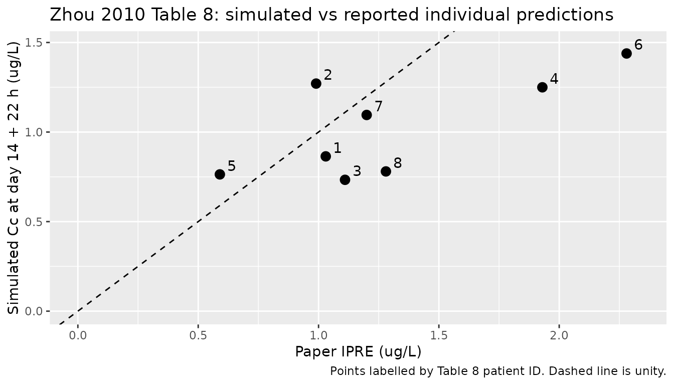
Replicate Cl/F covariate surfaces
The Discussion of Zhou 2010 reproduces the final-model formula
Cl/F = 5.9 x [1 - 0.412*SPI] x [1 - 0.0101*(WT - 62.9)] x [1 - 0.0012*(Cr - 126.8)].
The chunk below evaluates the formula analytically across the observed
WT and CREAT ranges so the multiplicative effects can be sanity-checked
against the in-file ini() coefficients.
typical_cl <- function(WT, CREAT, CONMED_SPIRON,
                       cl0 = 5.9, theta_spi = 0.412,
                       theta_wt = 0.0101, theta_cr = 0.00120,
                       WT_ref = 62.9, CREAT_ref = 126.8) {
  cl0 *
    (1 - theta_spi * CONMED_SPIRON) *
    (1 - theta_wt  * (WT    - WT_ref)) *
    (1 - theta_cr  * (CREAT - CREAT_ref))
}

cov_grid <- expand.grid(
  WT = seq(40, 90, by = 5),
  CREAT = seq(40, 400, by = 20),
  CONMED_SPIRON = c(0, 1)
) |>
  as_tibble() |>
  mutate(cl_typical = typical_cl(WT, CREAT, CONMED_SPIRON),
         SPI_label = ifelse(CONMED_SPIRON == 1, "On spironolactone", "Off spironolactone"))

ggplot(cov_grid, aes(CREAT, cl_typical, colour = factor(WT), group = WT)) +
  geom_line() +
  facet_wrap(~ SPI_label) +
  scale_colour_viridis_d(name = "Weight (kg)") +
  labs(x = "Serum creatinine (umol/L)",
       y = "Typical Cl/F (L/h)",
       title = "Zhou 2010 final-model Cl/F surface",
       caption = "Reproduces the Discussion's final-model Cl/F formula across the observed WT (34-91 kg) and CREAT (36-686 umol/L) ranges.")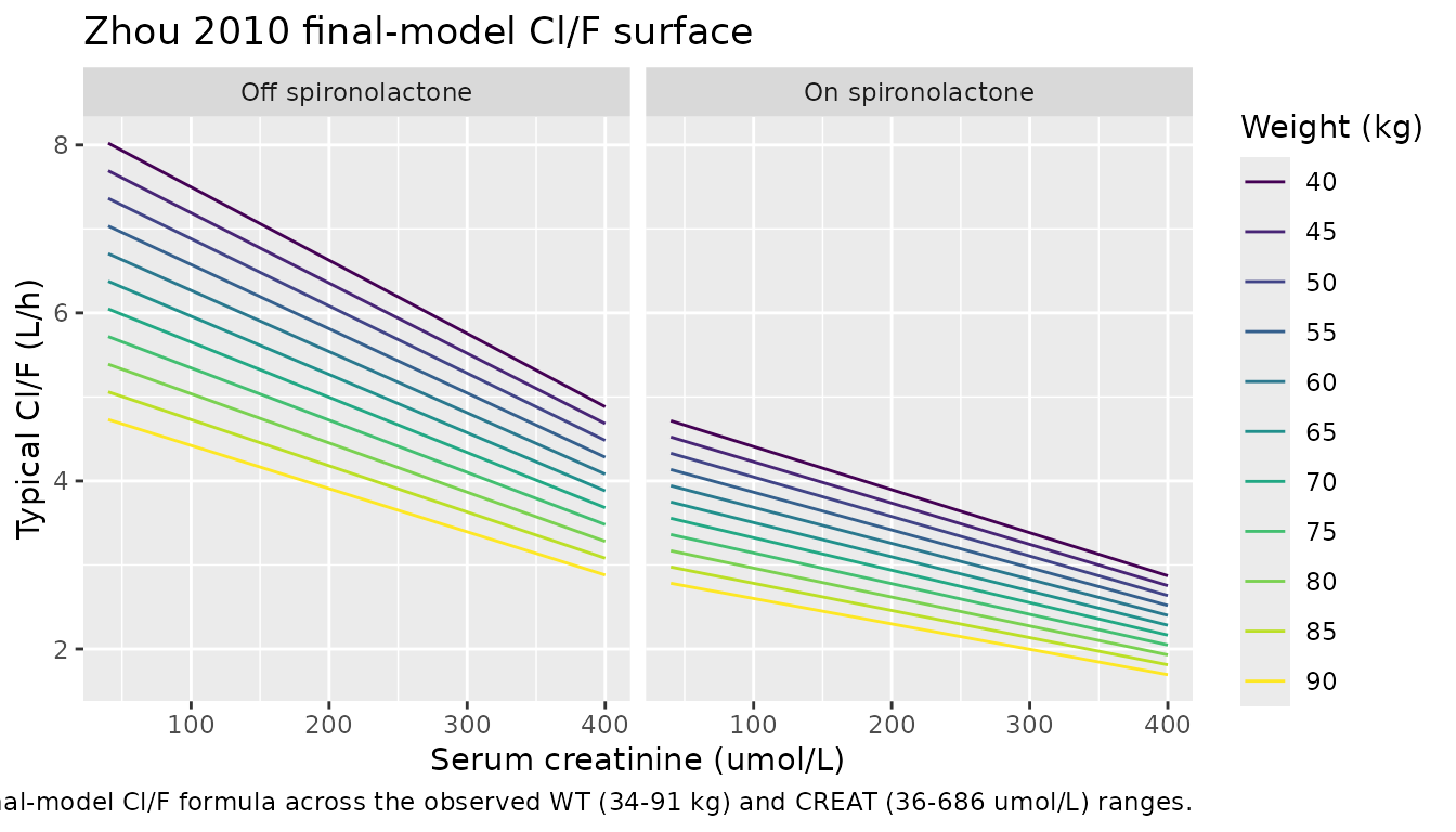
PKNCA single-dose validation
Zhou 2010 does not report any formal NCA-derived parameters (no Cmax
/ Tmax / AUC / half-life summaries appear in the article). The chunk
below runs PKNCA on a simulated single 0.125 mg oral dose for the
reference subject (WT = 62.9 kg, CREAT = 126.8 umol/L, no
spironolactone) as a sanity-check that the model produces non-negative,
dimensionally consistent serum concentrations with a half-life close to
the canonical digoxin half-life of 36-48 h
(t1/2 = ln(2) * V / CL = ln(2) * 550 / 5.9 ~= 64.6 h at the
typical subject; consistent with the upper end of the published range
for elderly patients).
single_dose_evt <- rxode2::et(amt = 0.125, cmt = "depot") |>
  rxode2::et(seq(0, 192, by = 0.25))
single_dose_evt <- as.data.frame(single_dose_evt)
single_dose_evt$id <- 1L
single_dose_evt$WT <- 62.9
single_dose_evt$CREAT <- 126.8
single_dose_evt$CONMED_SPIRON <- 0L
single_dose_evt$treatment <- "single 0.125 mg oral, typical subject"

sim_single <- rxode2::rxSolve(
  rxode2::zeroRe(mod),
  events = single_dose_evt,
  keep   = c("WT", "CREAT", "CONMED_SPIRON", "treatment")
) |>
  as.data.frame()
#> ℹ parameter labels from comments will be replaced by 'label()'
#> ℹ omega/sigma items treated as zero: 'etalcl', 'etalvc'

if (!"id" %in% names(sim_single)) sim_single$id <- 1L

sim_nca <- sim_single |>
  filter(!is.na(Cc)) |>
  select(id, time, Cc, treatment)

conc_obj <- PKNCA::PKNCAconc(sim_nca, Cc ~ time | treatment + id)

dose_df <- single_dose_evt |>
  filter(evid == 1L) |>
  select(id, time, amt, treatment)

dose_obj <- PKNCA::PKNCAdose(dose_df, amt ~ time | treatment + id)

intervals <- data.frame(
  start      = 0,
  end        = Inf,
  cmax       = TRUE,
  tmax       = TRUE,
  aucinf.obs = TRUE,
  half.life  = TRUE
)

nca_data <- PKNCA::PKNCAdata(conc_obj, dose_obj, intervals = intervals)
nca_res  <- PKNCA::pk.nca(nca_data)

knitr::kable(
  as.data.frame(nca_res$result),
  digits  = 4,
  caption = "Simulated single 0.125 mg oral PKNCA output for the Zhou 2010 reference subject (WT = 62.9 kg, CREAT = 126.8 umol/L, no spironolactone)."
)| treatment | id | start | end | PPTESTCD | PPORRES | exclude |
|---|---|---|---|---|---|---|
| single 0.125 mg oral, typical subject | 1 | 0 | Inf | cmax | 0.2198 | NA |
| single 0.125 mg oral, typical subject | 1 | 0 | Inf | tmax | 3.0000 | NA |
| single 0.125 mg oral, typical subject | 1 | 0 | Inf | tlast | 192.0000 | NA |
| single 0.125 mg oral, typical subject | 1 | 0 | Inf | clast.obs | 0.0292 | NA |
| single 0.125 mg oral, typical subject | 1 | 0 | Inf | lambda.z | 0.0107 | NA |
| single 0.125 mg oral, typical subject | 1 | 0 | Inf | r.squared | 1.0000 | NA |
| single 0.125 mg oral, typical subject | 1 | 0 | Inf | adj.r.squared | 1.0000 | NA |
| single 0.125 mg oral, typical subject | 1 | 0 | Inf | lambda.z.time.first | 3.2500 | NA |
| single 0.125 mg oral, typical subject | 1 | 0 | Inf | lambda.z.time.last | 192.0000 | NA |
| single 0.125 mg oral, typical subject | 1 | 0 | Inf | lambda.z.n.points | 756.0000 | NA |
| single 0.125 mg oral, typical subject | 1 | 0 | Inf | clast.pred | 0.0292 | NA |
| single 0.125 mg oral, typical subject | 1 | 0 | Inf | half.life | 64.6193 | NA |
| single 0.125 mg oral, typical subject | 1 | 0 | Inf | span.ratio | 2.9210 | NA |
| single 0.125 mg oral, typical subject | 1 | 0 | Inf | aucinf.obs | 21.1847 | NA |
Assumptions and deviations
-
Residual error is additive-only in the final model.
Zhou 2010 Table 2 (basic model) reports both proportional (CV) and
additive (SD) residual terms, consistent with the basic-model equation
Y = YPRED + YPRED * ERR(1) + ERR(2). Tables 5 and 7 (full-regression and final models) both record the proportional CV as “-” with only an additive SD value (0.365 ug/L in the final model). This is read as the proportional term having been dropped during covariate-model refinement; the model file therefore implementsCc ~ add(addSd)withaddSd = 0.365. -
Ka and Ka IIV are fixed. The paper’s Results
section (Basic model) states: “Because the absorption phase in the data
had been completed, Ka and inter-individual variation were fixed to 1.63
h-1 and 0, respectively, in the next calculation to avoid the effect of
Ka fluctuation on the stability of model.”
lkais therefore wrapped infixed()andetalkais omitted from the IIV block. -
Covariate-effect sign convention. The final-model
formula reported in the Discussion uses positive coefficients with
(1 - theta * cov)multiplicative linear-deviation factors. The model file preserves the paper-reported positive signs oftheta_SPI-Cl = 0.412,theta_WT-Cl = 0.0101, andtheta_Cr-Cl = 0.00120; the minus signs appear explicitly inmodel()so the in-fileini()value matches the source table verbatim. -
WT effect coefficient is statistically marginal but
retained. Table 7 reports
theta_WT-Cl = 0.0101with RSE 120% and 95% CI -0.0136 to 0.0338 – the confidence interval crosses zero. Zhou 2010 retained the WT-Cl term in the final model on the strength of the backward-elimination dOFV criterion (7.515 > 6.63 at the 0.01 level; Table 6); the model file therefore retains it as the published final model rather than dropping it on the 95% CI argument. - Reference covariate values are population means, not medians. Table 1 reports means (62.9 kg WT, 126.8 umol/L CREAT) and not medians; the Discussion formula and the model file use those means as the reference values, matching the source.
- No NCA values published. Zhou 2010 reports population Cl/F and Vd/F estimates but not Cmax / Tmax / AUC / half-life. The PKNCA section above is a sanity check on the implementation; it is not a comparison to a published NCA table.
- Table 8 IPRE vs simulated typical-value. Table 8 reports individual-predicted (IPRE) concentrations from the NONMEM fit. The vignette compares the simulated day-14 22-h post-dose concentration (zero-eta, per-subject covariates) against IPRE. The exact phlebotomy time is not reported per patient in Table 8 (only the cohort-level median 22.9 h post-dose from Table 1), so the simulated time is an approximation; some scatter around the unity line is expected and is documented in the Table 8 comparison plot above.
-
Population field
assay. The paper reports fluorescence polarization immunoassay on Abbott TDx-FLx with a 0.2 ug/L LLOQ; this is recorded inpopulation$assayrather than the canonical schema so the assay context is searchable viareadModelDb("Zhou_2010_digoxin")$population.