SGLT2 inhibitors: PK, urinary glucose excretion, FPG and HbA1c (Yao 2023) • nlmixr2lib

Model and source

Yao 2023 is a model-based meta-analysis (MBMA) of the three globally marketed sodium-glucose co-transporter-2 (SGLT2) inhibitors available when the literature search closed. It builds a chain that starts at dose and ends at a disease endpoint:

dose -> PK (per drug) -> AUC(0-24 h) at steady state
     -> dUGEc (shared Emax, drug-specific EC50)
     -> FPG (linear in dUGEc)
     -> HbA1c (indirect-response turnover driven by FPG)

The paper fits this chain sequentially, because the PK, PD and endpoint data come from different studies and different subjects. The extraction mirrors that structure: three independent population PK models, one per drug, plus one class-level PK/PD/endpoint model that the three feed through their steady-state AUC.

pk_models <- c(
  dapagliflozin = "Yao_2023_dapagliflozin_mbma",
  canagliflozin = "Yao_2023_canagliflozin_mbma",
  empagliflozin = "Yao_2023_empagliflozin_mbma"
)

# readModelDb() returns the model FUNCTION; rxode2::rxode() resolves it to a
# ui object whose metadata fields can be read directly.
pk_ui <- lapply(pk_models, function(nm) rxode2::rxode(readModelDb(nm)))
#> ℹ parameter labels from comments will be replaced by 'label()'
#> ℹ parameter labels from comments will be replaced by 'label()'
#> ℹ parameter labels from comments will be replaced by 'label()'
ep_ui <- rxode2::rxode(readModelDb("Yao_2023_sglt2_endpoints_mbma"))
#> ℹ parameter labels from comments will be replaced by 'label()'

Citation: Yao X, Zhou J, Song L, Ren Y, Hu P, Liu D. A model-based meta analysis study of sodium glucose co-transporter-2 inhibitors. CPT Pharmacometrics Syst Pharmacol. 2023;12(4):487-499. doi:10.1002/psp4.12934.
Article: https://doi.org/10.1002/psp4.12934
Supplement (Appendix S1, Tables S1-S2, Figures S1-S8): https://doi.org/10.1002/psp4.12934 (Supporting Information, file psp4-12-487-s001.docx)
Models contributed by this paper:

The four model files extracted from Yao 2023.
Model	Role
Yao_2023_dapagliflozin_mbma	Dapagliflozin population PK (2 transit compartments; food effect on Kt)
Yao_2023_canagliflozin_mbma	Canagliflozin population PK (4 transit compartments)
Yao_2023_empagliflozin_mbma	Empagliflozin population PK (2 transit compartments)
Yao_2023_sglt2_endpoints_mbma	Class-level AUC -> dUGEc -> FPG -> HbA1c endpoint model

Population

The PK layer pools 880 summary-level plasma concentrations from published dapagliflozin, canagliflozin and empagliflozin studies: 201 dapagliflozin subjects (177 healthy), 158 canagliflozin subjects (76 healthy) and 204 empagliflozin subjects (122 healthy). Mean age ranges from 38.1 to 46.8 years and mean body weight from 73.3 to 76.4 kg across the three PK datasets (Yao 2023 Table S2).

The endpoint layer pools 848 FPG and 1219 HbA1c study-arm means from 80 trials in adults with type 2 diabetes: 8324 dapagliflozin, 7004 canagliflozin and 9489 empagliflozin patients (Yao 2023 Table S1). Those cohorts are older and heavier than the PK cohorts (mean age 55.8-57.6 years, mean weight 79.0-84.9 kg) with a mean baseline FPG near 160 mg/dL and a mean baseline HbA1c near 7.9% (Table S2). Trials in patients with moderate or severe renal impairment or hepatic insufficiency were excluded, as were trials using insulin, so the model applies to patients with a glomerular filtration rate above 60 mL/min/1.73 m^2 – a limitation the authors state explicitly.

Because this is a meta-analysis, the unit of observation is a published study-arm mean, not an individual measurement. Every variance term in every one of the four models is therefore a BETWEEN-STUDY variance, encoded as eta_study_*. These models simulate study-arm mean trajectories; they are not individual-subject models and must not be used as such.

Endpoint-model population metadata.
Field	Value
Species	human
Patients	24,817
Studies	80
Disease state	Type 2 diabetes mellitus with normal or mildly impaired renal function (glomerular filtration rate above 60 mL/min/1.73 m2). Studies in patients with moderate or severe kidney impairment or hepatic insufficiency were excluded, as were trials using insulin. Baseline FPG about 160 mg/dL and baseline HbA1c about 7.9%.
Dose range	Placebo plus dapagliflozin 1-50 mg, canagliflozin 50-300 mg and empagliflozin 1-100 mg once daily; treatment durations up to 104 weeks (Yao 2023 Table S1)

Source trace

Every ini() entry carries an in-file comment naming its source location. The table below collects them.

Source trace for every model equation and parameter.
Quantity	Value	Source
PK ODEs (2 transit + 2 compartment)	structure	Appendix S1 Eq. S1-S5
PK ODEs, canagliflozin (4 transit + 2 compartment)	structure	Appendix S1 Eq. S6-S12
Inter-study variability model	P = theta * exp(eta)	Appendix S1 Eq. S13
Residual error model	Y = F + Feps1W + eps2*W	Appendix S1 Eq. S14
Dapagliflozin CL/F, Vc/F, CLD/F, VT/F, Kt	19.5, 82.0, 10.3, 122, 6.50	Table 1
Dapagliflozin food effect on Kt	0.254	Table 1 (Fed)
Canagliflozin CL/F, Vc/F, CLD/F, VT/F, Kt	12.0, 85.5, 9.77, 108, 6.38	Table 1
Empagliflozin CL/F, Vc/F, CLD/F, VT/F, Kt	4.25, 30.6, 1.37, 28.3, 4.13	Table 1
dUGEc definition	(UGE - UGE_base) / FPG_base	Equation 1
dUGEc Emax model	Emax * AUC / (EC50 + AUC)	Equation 2
Emax (shared across the three drugs)	0.606 g/(mg/dL)	Table 2
EC50 dapa / cana / empa	56.6 / 2310 / 841 ng*h/mL	Table 2
FPG placebo model	FPGbase + Pfmax(1-exp(-Kfpt)) + DISfp*t	Equation 3
FPG drug model	FPG_placebo + SLOPEfd * dUGEc	Equation 4 (see Errata)
FPG baseline; Pfmax1-4	160; 1.45, 1.90, -1.37, 4.30 mg/dL	Table 2
Kfp; DISfp; SLOPEfd	0.340 /week; 3.13 mg/dL/100wk; -43.3	Table 2
HbA1c placebo model	HbA1cbase - Phmax(1-exp(-Khpt)) + DIShp*t	Equation 5 (see Errata)
Kin definition	Kout * HbA1cbase - Kin2	Equation 6
HbA1c drug ODE	FPG/FPGbaseKin + Kin2 - KoutHbA1c	Equation 7
HbA1c total	HbA1c_placebo + HbA1c_drug	Equation 8
HbA1c baseline; Phmax1-4	7.92; -0.200, 0.0510, -0.230, -0.06 %	Table 2
Khp; DIShp; Kout; Kin2	0.240 /week; 0.310 %/100wk; 0.200 /week; 0.500 %/week	Table 2
Residual variances (PK, PK/PD, FPG, HbA1c)	0.457/0.462; 0.222/0.0646; 0.0330; 0.006	Tables 1-2

Part 1 - Pharmacokinetics

Typical-value profiles at the label doses

# Typical-value solve: zeroRe() removes both the between-study eta terms and
# the residual error, leaving the population prediction.
solve_typical <- function(model_name, events, keep = character()) {
  mod <- rxode2::zeroRe(readModelDb(model_name))
  out <- rxode2::rxSolve(mod, events, keep = keep, returnType = "data.frame")
  if (is.null(out$id)) out$id <- 1L
  out
}

# Observation rows are placed on the "central" ODE STATE, never on the "Cc"
# observable: referencing an observable as a compartment renumbers the
# compartment slots. rxode2 returns Cc as a column at these rows anyway.
pk_events <- function(dose_mg, n_days, obs_times, fed = 0) {
  dosing <- data.frame(
    id = 1L, time = seq(0, by = 24, length.out = n_days),
    amt = dose_mg, evid = 1L, cmt = "depot", FED = fed
  )
  obs <- data.frame(
    id = 1L, time = obs_times, amt = NA_real_, evid = 0L,
    cmt = "central", FED = fed
  )
  dplyr::arrange(dplyr::bind_rows(dosing, obs), time, dplyr::desc(evid))
}

label_dose <- c(dapagliflozin = 10, canagliflozin = 300, empagliflozin = 25)

profile_times <- sort(unique(c(seq(0, 48, by = 0.1))))

pk_profiles <- dplyr::bind_rows(lapply(names(pk_models), function(drug) {
  ev <- pk_events(label_dose[[drug]], n_days = 2, obs_times = profile_times)
  # rxSolve() returns one row per OBSERVATION record; dosing records produce no
  # output row, so no evid filter is needed (and evid is not a returned column).
  solve_typical(pk_models[[drug]], ev) |>
    dplyr::mutate(drug = drug)
}))
#> ℹ parameter labels from comments will be replaced by 'label()'
#> ℹ omega/sigma items treated as zero: 'eta_study_lcl', 'eta_study_lvc', 'eta_study_lvp', 'eta_study_lktr'
#> ℹ parameter labels from comments will be replaced by 'label()'
#> ℹ omega/sigma items treated as zero: 'eta_study_lcl', 'eta_study_lvc', 'eta_study_lq', 'eta_study_lvp', 'eta_study_lktr'
#> ℹ parameter labels from comments will be replaced by 'label()'
#> ℹ omega/sigma items treated as zero: 'eta_study_lcl', 'eta_study_lvc', 'eta_study_lvp', 'eta_study_lktr'

ggplot(pk_profiles, aes(time, Cc, colour = drug)) +
  geom_line(linewidth = 0.8) +
  scale_y_log10() +
  labs(
    x = "Time (h)", y = "Plasma concentration (ng/mL)", colour = NULL,
    title = "Typical-value profiles at the label dose, first two daily doses",
    subtitle = "Dapagliflozin 10 mg, canagliflozin 300 mg, empagliflozin 25 mg"
  ) +
  theme_bw()
#> Warning in scale_y_log10(): log-10 transformation introduced infinite values.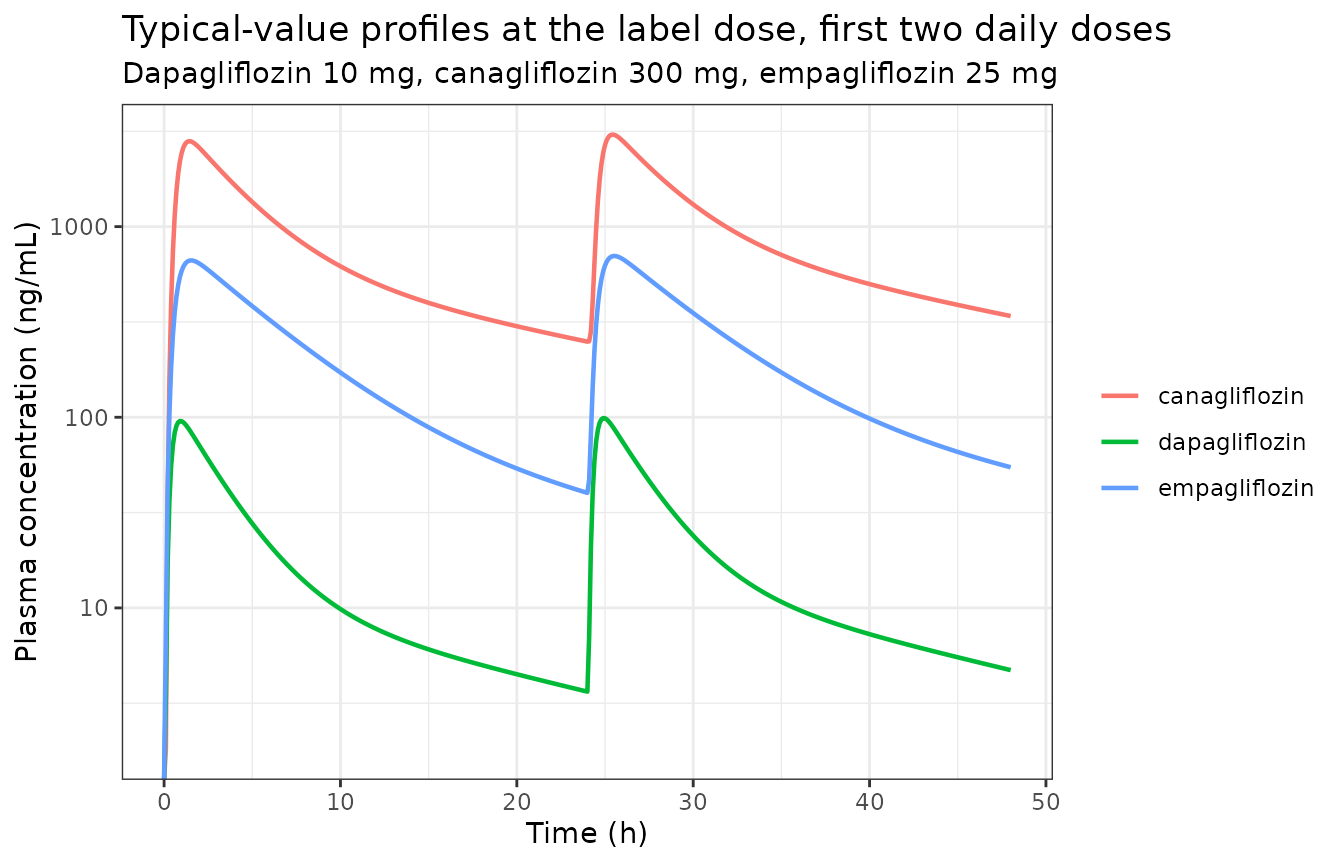

The three profiles reproduce the qualitative features Yao 2023 reports in Figure S3 and the Discussion: a fast transit-limited absorption phase, a peak inside the first two hours, and a terminal phase slow enough to give modest accumulation on once-daily dosing.

The dapagliflozin food effect

Food is the only covariate retained anywhere in the PK layer. Yao 2023 Table 1 reports the coefficient as a bare multiplier of 0.254 on the transit rate constant, and the Discussion states that food “could significantly influence the Kt parameter (p < 0.005) in dapagliflozin, which is consistent with a longer time to maximum concentration of dapagliflozin under fed condition.”

food_times <- seq(0, 24, by = 0.05)
food <- dplyr::bind_rows(lapply(c(fasted = 0, fed = 1), function(f) {
  ev <- pk_events(10, n_days = 1, obs_times = food_times, fed = f)
  solve_typical("Yao_2023_dapagliflozin_mbma", ev, keep = "FED")
})) |>
  dplyr::mutate(state = ifelse(FED == 1, "fed", "fasted"))
#> ℹ parameter labels from comments will be replaced by 'label()'
#> ℹ omega/sigma items treated as zero: 'eta_study_lcl', 'eta_study_lvc', 'eta_study_lvp', 'eta_study_lktr'
#> ℹ parameter labels from comments will be replaced by 'label()'
#> ℹ omega/sigma items treated as zero: 'eta_study_lcl', 'eta_study_lvc', 'eta_study_lvp', 'eta_study_lktr'

food_summary <- food |>
  dplyr::group_by(state) |>
  dplyr::summarise(
    Tmax_h = time[which.max(Cc)],
    Cmax_ng_mL = max(Cc),
    .groups = "drop"
  )
knitr::kable(
  food_summary,
  digits = 2,
  caption = "Dapagliflozin 10 mg single dose: the fed state delays and blunts the peak."
)

Dapagliflozin 10 mg single dose: the fed state delays and blunts the peak.
state	Tmax_h	Cmax_ng_mL
fasted	0.95	95.6
fed	2.70	65.7


# Deterministic (typical-value) quantities, so an exact bound is appropriate.
stopifnot(
  # Food must DELAY the peak, which is the direction the paper reports.
  food_summary$Tmax_h[food_summary$state == "fed"] >
    food_summary$Tmax_h[food_summary$state == "fasted"],
  # Food must LOWER the peak (slower input into an unchanged clearance).
  food_summary$Cmax_ng_mL[food_summary$state == "fed"] <
    food_summary$Cmax_ng_mL[food_summary$state == "fasted"]
)

Steady-state AUC(0-24 h): an exact internal identity, and the published values

For a linear model at steady state the AUC over one dosing interval is exactly daily dose / CL. The endpoint model consumes precisely that quantity, so the identity is worth checking with a real NCA rather than assuming it.

Yao 2023 Results reports “the steady-state AUC in 24 h after long-term treatment was 51.39 ng/mLh for dapagliflozin, 83.6 ng/mLh for canagliflozin, and 235.3 ng/mLh for empagliflozin.” Those values are far too small to be whole-dose exposures – dapagliflozin 10 mg gives roughly 500-600 ngh/mL – but they match 1000 / CL for each drug to within a few tenths of a percent, i.e. they are dose-normalised: AUC(0-24 h) at steady state per mg of daily dose. The printed unit omits the /mg. Simulating a 1 mg once-daily regimen to steady state and running PKNCA over the final dosing interval therefore tests the transcription of every PK parameter that determines exposure.

tau <- 24
n_days_ss <- 21
start_ss <- (n_days_ss - 1) * tau
end_ss <- start_ss + tau

# Coarse sampling through the accumulation phase, dense sampling over the
# final interval so the trapezoidal AUC resolves the peak.
nca_times <- sort(unique(c(
  seq(0, start_ss, by = 4),
  seq(start_ss, end_ss, by = 0.05)
)))

nca_input <- dplyr::bind_rows(lapply(names(pk_models), function(drug) {
  ev <- pk_events(1, n_days = n_days_ss, obs_times = nca_times)
  solve_typical(pk_models[[drug]], ev) |>
    dplyr::mutate(treatment = drug, id = 1L)
}))
#> ℹ parameter labels from comments will be replaced by 'label()'
#> ℹ omega/sigma items treated as zero: 'eta_study_lcl', 'eta_study_lvc', 'eta_study_lvp', 'eta_study_lktr'
#> ℹ parameter labels from comments will be replaced by 'label()'
#> ℹ omega/sigma items treated as zero: 'eta_study_lcl', 'eta_study_lvc', 'eta_study_lq', 'eta_study_lvp', 'eta_study_lktr'
#> ℹ parameter labels from comments will be replaced by 'label()'
#> ℹ omega/sigma items treated as zero: 'eta_study_lcl', 'eta_study_lvc', 'eta_study_lvp', 'eta_study_lktr'

# The PKNCA input filter is !is.na(Cc) ONLY: filtering on time or on Cc > 0
# would drop the interval-start record and trigger the "AUC range starting
# before the first measurement" warning.
conc_df <- nca_input |>
  dplyr::filter(!is.na(Cc)) |>
  dplyr::select(id, time, Cc, treatment)

dose_df <- dplyr::bind_rows(lapply(names(pk_models), function(drug) {
  data.frame(
    id = 1L, time = seq(0, by = tau, length.out = n_days_ss),
    amt = 1, treatment = drug
  )
}))

conc_obj <- PKNCA::PKNCAconc(conc_df, Cc ~ time | treatment + id,
                             concu = "ng/mL", timeu = "h")
dose_obj <- PKNCA::PKNCAdose(dose_df, amt ~ time | treatment + id,
                             doseu = "mg")

intervals <- data.frame(
  start = start_ss, end = end_ss,
  cmax = TRUE, tmax = TRUE, auclast = TRUE, cav = TRUE
)

nca_res <- PKNCA::pk.nca(PKNCA::PKNCAdata(conc_obj, dose_obj, intervals = intervals))

published_auc <- tibble::tribble(
  ~treatment,      ~auclast,
  "dapagliflozin",   51.39,
  "canagliflozin",   83.60,
  "empagliflozin",  235.30
)

cmp <- nlmixr2lib::ncaComparisonTable(
  simulated = nca_res,
  reference = published_auc,
  by = "treatment",
  units = c(auclast = "ng*h/mL per mg/day"),
  tolerance_pct = 20
)
knitr::kable(
  cmp,
  caption = paste(
    "Simulated steady-state AUC(0-24 h) at 1 mg once daily versus the",
    "dose-normalised values reported in Yao 2023 Results.",
    "* differs from reference by more than 20%."
  ),
  align = c("l", "l", "r", "r", "r")
)

Simulated steady-state AUC(0-24 h) at 1 mg once daily versus the dose-normalised values reported in Yao 2023 Results. * differs from reference by more than 20%.
NCA parameter	treatment	Reference	Simulated	% diff
AUClast (ng*h/mL per mg/day)	dapagliflozin	51.4	51.3	-0.2%
AUClast (ng*h/mL per mg/day)	canagliflozin	83.6	83.3	-0.3%
AUClast (ng*h/mL per mg/day)	empagliflozin	235	235	-0.0%

auc_sim <- as.data.frame(nca_res$result) |>
  dplyr::filter(PPTESTCD == "auclast") |>
  dplyr::select(treatment, auclast = PPORRES)

check_auc <- auc_sim |>
  dplyr::left_join(published_auc, by = "treatment",
                   suffix = c("_sim", "_pub")) |>
  dplyr::mutate(
    cl_L_per_h = vapply(
      treatment,
      function(d) exp(pk_ui[[d]]$theta[["lcl"]]),
      numeric(1)
    ),
    auc_identity = 1000 / cl_L_per_h,
    pct_vs_identity = 100 * (auclast_sim / auc_identity - 1),
    pct_vs_published = 100 * (auclast_sim / auclast_pub - 1)
  )

knitr::kable(
  check_auc |>
    dplyr::rename(
      "Drug" = treatment,
      "AUC simulated" = auclast_sim,
      "AUC published" = auclast_pub,
      "CL/F (L/h)" = cl_L_per_h,
      "1000 / CL" = auc_identity,
      "% vs identity" = pct_vs_identity,
      "% vs published" = pct_vs_published
    ),
  digits = 3,
  caption = "The PKNCA AUC reproduces both the closed-form identity and the published dose-normalised value."
)

The PKNCA AUC reproduces both the closed-form identity and the published dose-normalised value.
Drug	AUC simulated	AUC published	CL/F (L/h)	1000 / CL	% vs identity	% vs published
canagliflozin	83.333	83.60	12.00	83.333	0.000	-0.319
dapagliflozin	51.282	51.39	19.50	51.282	-0.001	-0.211
empagliflozin	235.293	235.30	4.25	235.294	0.000	-0.003


# Both sides are deterministic typical-value quantities (zeroRe(), fixed time
# grid), so exact bounds are appropriate here: no cohort is drawn, and the only
# error is trapezoidal discretisation of a smooth curve.
stopifnot(
  # NCA versus the closed form dose/CL: pure numerical integration error.
  max(abs(check_auc$pct_vs_identity)) < 0.5,
  # NCA versus the paper's own printed numbers: confirms CL was transcribed
  # correctly for all three drugs AND that the printed values are per mg/day.
  max(abs(check_auc$pct_vs_published)) < 1
)

Both bounds hold: the numerical AUC agrees with 1000 / CL to well under a percent, and matches all three published values to under 1%. That settles the unit reading and validates the clearance transcription for every drug.

Part 2 - Exposure to the translational biomarker dUGEc

Yao 2023 Equation 2 gives the biomarker as a shared-Emax, drug-specific-EC50 function of steady-state exposure. Because dUGEc has no dynamics, it can be read straight off the endpoint model by solving it once per exposure level.

ep_events <- function(cov_rows, times) {
  cov_rows$.row <- seq_len(nrow(cov_rows))
  tidyr::crossing(cov_rows, time = times) |>
    dplyr::mutate(
      id = .row,
      amt = NA_real_,
      evid = 0L,
      # cmt names the ODE STATE (never an observable). The endpoint model has
      # three observation endpoints (UGEc, FPG, HbA1c), so rxode2 also needs a
      # dvid to resolve the dvid->cmt mapping; dvid = 1 selects UGEc, and every
      # observable is returned as its own column regardless.
      cmt = "hba1c_drug",
      dvid = 1L
    ) |>
    dplyr::select(-.row) |>
    dplyr::arrange(id, time) |>
    as.data.frame()
}

strata_cols <- function(stratum) {
  data.frame(
    TRT_T2DM_NAIVE = as.integer(stratum == "naive"),
    TRT_T2DM_NONNAIVE = as.integer(stratum == "non-naive"),
    TRT_T2DM_ADDON = as.integer(stratum == "add-on"),
    TRT_T2DM_MIXED = as.integer(stratum == "mixed")
  )
}

# AUC covariate row for one arm: only the treated drug's column is non-zero.
auc_cols <- function(drug, auc) {
  data.frame(
    AUC_DAPA = ifelse(drug == "dapagliflozin", auc, 0),
    AUC_CANA = ifelse(drug == "canagliflozin", auc, 0),
    AUC_EMPA = ifelse(drug == "empagliflozin", auc, 0)
  )
}

solve_endpoints <- function(cov_rows, times, keep) {
  mod <- rxode2::zeroRe(readModelDb("Yao_2023_sglt2_endpoints_mbma"))
  ev <- ep_events(cov_rows, times)
  out <- rxode2::rxSolve(mod, ev, keep = keep, returnType = "data.frame")
  if (is.null(out$id)) out$id <- 1L
  out
}

auc_grid <- 10^seq(1, 5, length.out = 60)

ugec_rows <- dplyr::bind_rows(lapply(names(pk_models), function(drug) {
  dplyr::bind_cols(
    data.frame(drug = drug, auc = auc_grid),
    auc_cols(drug, auc_grid),
    strata_cols("naive")[rep(1, length(auc_grid)), , drop = FALSE]
  )
}))

ugec_curve <- solve_endpoints(ugec_rows, times = 0, keep = c("drug", "auc"))
#> ℹ parameter labels from comments will be replaced by 'label()'
#> ℹ omega/sigma items treated as zero: 'eta_study_pfmax_naive', 'eta_study_pfmax_addon', 'eta_study_pfmax_mixed', 'eta_study_phmax_naive', 'eta_study_phmax_addon', 'eta_study_phmax_mixed', 'eta_study_lrbase_fpg', 'eta_study_lkfp', 'eta_study_slopefd', 'eta_study_lrbase_hba1c', 'eta_study_lkhp', 'eta_study_dishp', 'eta_study_lkout'
#> Warning: multi-subject simulation without without 'omega'

ggplot(ugec_curve, aes(auc, UGEc, colour = drug)) +
  geom_line(linewidth = 0.8) +
  scale_x_log10() +
  labs(
    x = "AUC(0-24 h) at steady state (ng*h/mL)",
    y = expression(Delta * "UGEc  (g/(mg/dL))"),
    colour = NULL,
    title = "Replicates Figure 2 of Yao 2023",
    subtitle = "Shared Emax of 0.606; EC50 56.6 / 2310 / 841 ng*h/mL"
  ) +
  theme_bw()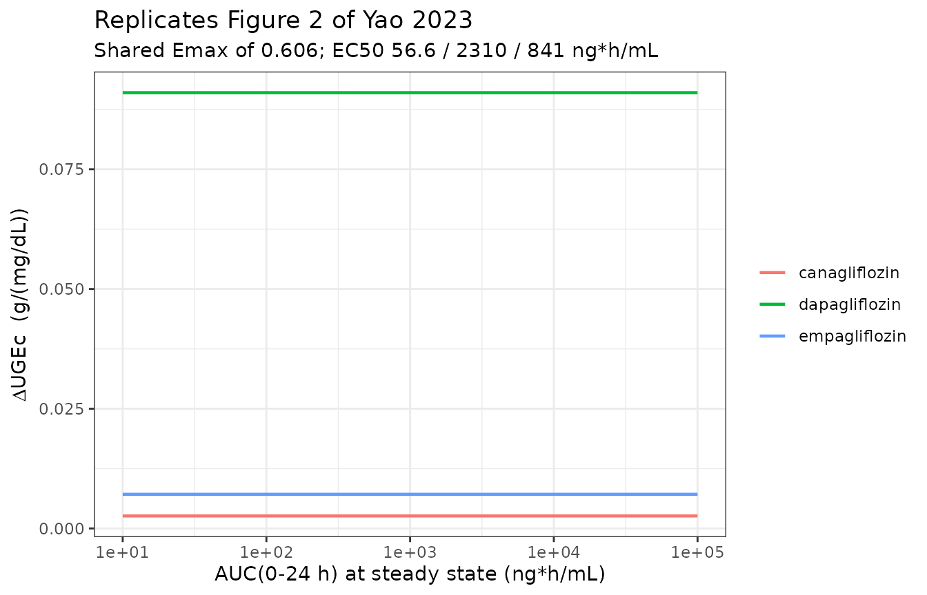

ec50_pub <- c(dapagliflozin = 56.6, canagliflozin = 2310, empagliflozin = 841)
emax_pub <- 0.606

ugec_at <- function(drug, auc) {
  row <- dplyr::bind_cols(
    auc_cols(drug, auc),
    strata_cols("naive")[rep(1, length(auc)), , drop = FALSE]
  )
  solve_endpoints(row, times = 0, keep = character())$UGEc
}

# At AUC = EC50 the Emax expression must give exactly half of Emax, for every
# drug. This is a structural identity, so an exact bound is right.
half_max <- vapply(names(ec50_pub), function(d) ugec_at(d, ec50_pub[[d]]), numeric(1))
#> ℹ parameter labels from comments will be replaced by 'label()'
#> ℹ omega/sigma items treated as zero: 'eta_study_pfmax_naive', 'eta_study_pfmax_addon', 'eta_study_pfmax_mixed', 'eta_study_phmax_naive', 'eta_study_phmax_addon', 'eta_study_phmax_mixed', 'eta_study_lrbase_fpg', 'eta_study_lkfp', 'eta_study_slopefd', 'eta_study_lrbase_hba1c', 'eta_study_lkhp', 'eta_study_dishp', 'eta_study_lkout'
#> ℹ parameter labels from comments will be replaced by 'label()'
#> ℹ omega/sigma items treated as zero: 'eta_study_pfmax_naive', 'eta_study_pfmax_addon', 'eta_study_pfmax_mixed', 'eta_study_phmax_naive', 'eta_study_phmax_addon', 'eta_study_phmax_mixed', 'eta_study_lrbase_fpg', 'eta_study_lkfp', 'eta_study_slopefd', 'eta_study_lrbase_hba1c', 'eta_study_lkhp', 'eta_study_dishp', 'eta_study_lkout'
#> ℹ parameter labels from comments will be replaced by 'label()'
#> ℹ omega/sigma items treated as zero: 'eta_study_pfmax_naive', 'eta_study_pfmax_addon', 'eta_study_pfmax_mixed', 'eta_study_phmax_naive', 'eta_study_phmax_addon', 'eta_study_phmax_mixed', 'eta_study_lrbase_fpg', 'eta_study_lkfp', 'eta_study_slopefd', 'eta_study_lrbase_hba1c', 'eta_study_lkhp', 'eta_study_dishp', 'eta_study_lkout'
stopifnot(max(abs(half_max / (emax_pub / 2) - 1)) < 1e-6)

# The asymptote must approach Emax and never exceed it.
asymptote <- vapply(names(ec50_pub), function(d) ugec_at(d, 1e9), numeric(1))
#> ℹ parameter labels from comments will be replaced by 'label()'
#> ℹ omega/sigma items treated as zero: 'eta_study_pfmax_naive', 'eta_study_pfmax_addon', 'eta_study_pfmax_mixed', 'eta_study_phmax_naive', 'eta_study_phmax_addon', 'eta_study_phmax_mixed', 'eta_study_lrbase_fpg', 'eta_study_lkfp', 'eta_study_slopefd', 'eta_study_lrbase_hba1c', 'eta_study_lkhp', 'eta_study_dishp', 'eta_study_lkout'
#> ℹ parameter labels from comments will be replaced by 'label()'
#> ℹ omega/sigma items treated as zero: 'eta_study_pfmax_naive', 'eta_study_pfmax_addon', 'eta_study_pfmax_mixed', 'eta_study_phmax_naive', 'eta_study_phmax_addon', 'eta_study_phmax_mixed', 'eta_study_lrbase_fpg', 'eta_study_lkfp', 'eta_study_slopefd', 'eta_study_lrbase_hba1c', 'eta_study_lkhp', 'eta_study_dishp', 'eta_study_lkout'
#> ℹ parameter labels from comments will be replaced by 'label()'
#> ℹ omega/sigma items treated as zero: 'eta_study_pfmax_naive', 'eta_study_pfmax_addon', 'eta_study_pfmax_mixed', 'eta_study_phmax_naive', 'eta_study_phmax_addon', 'eta_study_phmax_mixed', 'eta_study_lrbase_fpg', 'eta_study_lkfp', 'eta_study_slopefd', 'eta_study_lrbase_hba1c', 'eta_study_lkhp', 'eta_study_dishp', 'eta_study_lkout'
stopifnot(
  max(abs(asymptote / emax_pub - 1)) < 1e-4,
  max(ugec_curve$UGEc) <= emax_pub
)

# A placebo arm (every AUC column 0) must give exactly zero biomarker response.
stopifnot(abs(ugec_at("none", 0)) < 1e-12)
#> ℹ parameter labels from comments will be replaced by 'label()'
#> ℹ omega/sigma items treated as zero: 'eta_study_pfmax_naive', 'eta_study_pfmax_addon', 'eta_study_pfmax_mixed', 'eta_study_phmax_naive', 'eta_study_phmax_addon', 'eta_study_phmax_mixed', 'eta_study_lrbase_fpg', 'eta_study_lkfp', 'eta_study_slopefd', 'eta_study_lrbase_hba1c', 'eta_study_lkhp', 'eta_study_dishp', 'eta_study_lkout'

knitr::kable(
  data.frame(
    Drug = names(ec50_pub),
    "EC50 (ng*h/mL)" = unname(ec50_pub),
    "dUGEc at EC50" = unname(half_max),
    "Emax/2" = emax_pub / 2,
    check.names = FALSE
  ),
  digits = 4,
  caption = "The Emax structure is recovered exactly at each drug's published EC50."
)

The Emax structure is recovered exactly at each drug’s published EC50.
Drug	EC50 (ng*h/mL)	dUGEc at EC50	Emax/2
dapagliflozin	56.6	0.303	0.303
canagliflozin	2310.0	0.303	0.303
empagliflozin	841.0	0.303	0.303

Where the label doses sit on the exposure-response curve

auc_label <- vapply(
  names(pk_models),
  function(d) 1000 * label_dose[[d]] / exp(pk_ui[[d]]$theta[["lcl"]]),
  numeric(1)
)

label_tab <- data.frame(
  Drug = names(auc_label),
  "Daily dose (mg)" = unname(label_dose[names(auc_label)]),
  "AUC(0-24 h),ss (ng*h/mL)" = unname(auc_label),
  "dUGEc (g/(mg/dL))" = vapply(names(auc_label),
                               function(d) ugec_at(d, auc_label[[d]]), numeric(1)),
  check.names = FALSE
)
#> ℹ parameter labels from comments will be replaced by 'label()'
#> ℹ omega/sigma items treated as zero: 'eta_study_pfmax_naive', 'eta_study_pfmax_addon', 'eta_study_pfmax_mixed', 'eta_study_phmax_naive', 'eta_study_phmax_addon', 'eta_study_phmax_mixed', 'eta_study_lrbase_fpg', 'eta_study_lkfp', 'eta_study_slopefd', 'eta_study_lrbase_hba1c', 'eta_study_lkhp', 'eta_study_dishp', 'eta_study_lkout'
#> ℹ parameter labels from comments will be replaced by 'label()'
#> ℹ omega/sigma items treated as zero: 'eta_study_pfmax_naive', 'eta_study_pfmax_addon', 'eta_study_pfmax_mixed', 'eta_study_phmax_naive', 'eta_study_phmax_addon', 'eta_study_phmax_mixed', 'eta_study_lrbase_fpg', 'eta_study_lkfp', 'eta_study_slopefd', 'eta_study_lrbase_hba1c', 'eta_study_lkhp', 'eta_study_dishp', 'eta_study_lkout'
#> ℹ parameter labels from comments will be replaced by 'label()'
#> ℹ omega/sigma items treated as zero: 'eta_study_pfmax_naive', 'eta_study_pfmax_addon', 'eta_study_pfmax_mixed', 'eta_study_phmax_naive', 'eta_study_phmax_addon', 'eta_study_phmax_mixed', 'eta_study_lrbase_fpg', 'eta_study_lkfp', 'eta_study_slopefd', 'eta_study_lrbase_hba1c', 'eta_study_lkhp', 'eta_study_dishp', 'eta_study_lkout'
label_tab$"Fraction of Emax" <- label_tab$"dUGEc (g/(mg/dL))" / emax_pub

knitr::kable(
  label_tab, digits = c(0, 0, 0, 4, 3),
  caption = "At their label doses the three drugs sit at a similar point on the shared Emax curve."
)

At their label doses the three drugs sit at a similar point on the shared Emax curve.
	Drug	Daily dose (mg)	AUC(0-24 h),ss (ng*h/mL)	dUGEc (g/(mg/dL))	Fraction of Emax
dapagliflozin	dapagliflozin	10	513	0.5458	0.901
canagliflozin	canagliflozin	300	25000	0.5547	0.915
empagliflozin	empagliflozin	25	5882	0.5302	0.875


# The paper's central claim is that the three drugs reach a SIMILAR maximum
# response and differ only in potency. At label doses they should therefore
# land close together on the response axis even though their EC50 values span
# a 40-fold range. Deterministic, so a tight bound is appropriate.
stopifnot(
  diff(range(label_tab$"Fraction of Emax")) < 0.06,
  all(label_tab$"Fraction of Emax" > 0.5)
)

Part 3 - FPG and HbA1c endpoints

Placebo trajectories by treatment-history stratum

Yao 2023 estimates a separate maximal placebo effect on each endpoint in each of four treatment-history strata. Figure 3 panels (a), (b), (e) and (f) show the corresponding visual predictive checks.

weeks <- seq(0, 104, by = 1)
strata <- c("naive", "non-naive", "add-on", "mixed")

placebo_rows <- dplyr::bind_rows(lapply(strata, function(s) {
  dplyr::bind_cols(
    data.frame(stratum = s),
    auc_cols("none", 0),
    strata_cols(s)
  )
}))

placebo <- solve_endpoints(placebo_rows, weeks, keep = "stratum")
#> ℹ parameter labels from comments will be replaced by 'label()'
#> ℹ omega/sigma items treated as zero: 'eta_study_pfmax_naive', 'eta_study_pfmax_addon', 'eta_study_pfmax_mixed', 'eta_study_phmax_naive', 'eta_study_phmax_addon', 'eta_study_phmax_mixed', 'eta_study_lrbase_fpg', 'eta_study_lkfp', 'eta_study_slopefd', 'eta_study_lrbase_hba1c', 'eta_study_lkhp', 'eta_study_dishp', 'eta_study_lkout'
#> Warning: multi-subject simulation without without 'omega'

placebo_long <- placebo |>
  dplyr::select(stratum, time, FPG, HbA1c) |>
  tidyr::pivot_longer(c(FPG, HbA1c), names_to = "endpoint", values_to = "value")

ggplot(placebo_long, aes(time, value, colour = stratum)) +
  geom_line(linewidth = 0.8) +
  facet_wrap(~endpoint, scales = "free_y") +
  labs(
    x = "Time after first dose (weeks)", y = NULL, colour = "Treatment history",
    title = "Placebo trajectories, replicating Figure 3 panels (a), (b), (e) and (f)",
    subtitle = "FPG in mg/dL; HbA1c in %"
  ) +
  theme_bw()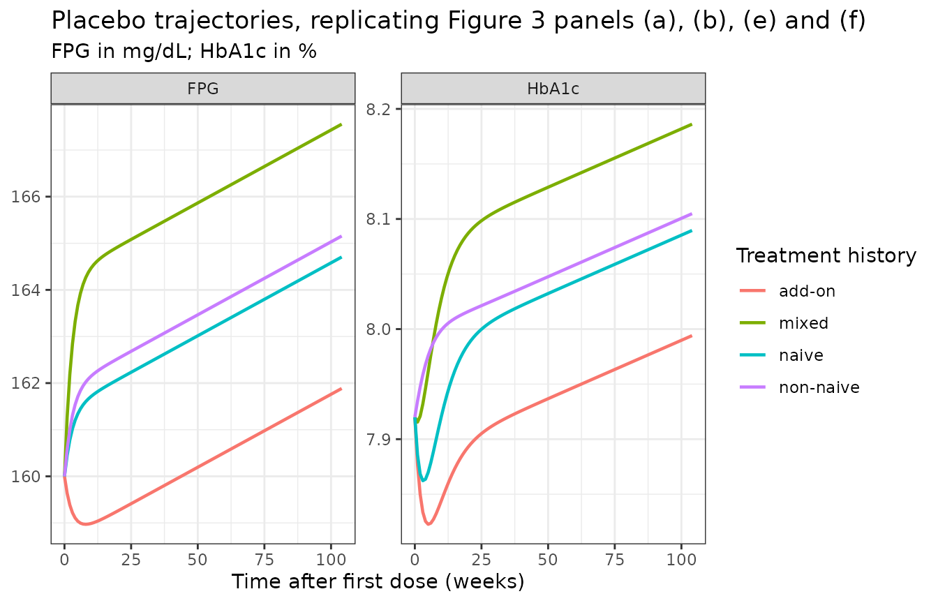

placebo_summary <- placebo |>
  dplyr::group_by(stratum) |>
  dplyr::summarise(
    fpg_0 = FPG[time == 0],
    fpg_min = min(FPG),
    fpg_104 = FPG[time == 104],
    hba1c_0 = HbA1c[time == 0],
    hba1c_min = min(HbA1c),
    hba1c_104 = HbA1c[time == 104],
    .groups = "drop"
  )
knitr::kable(placebo_summary, digits = 3,
             caption = "Placebo-arm endpoint summaries by treatment-history stratum.")

Placebo-arm endpoint summaries by treatment-history stratum.
stratum	fpg_0	fpg_min	fpg_104	hba1c_0	hba1c_min	hba1c_104
add-on	160	158.971	161.885	7.92	7.823	7.994
mixed	160	160.000	167.555	7.92	7.915	8.186
naive	160	160.000	164.705	7.92	7.862	8.090
non-naive	160	160.000	165.155	7.92	7.920	8.105


# Every arm must start exactly at the published baselines (Table 2).
stopifnot(
  max(abs(placebo_summary$fpg_0 - 160)) < 1e-8,
  max(abs(placebo_summary$hba1c_0 - 7.92)) < 1e-8
)

# The add-on stratum is the only one in which the placebo FPG effect is a
# DECREASE (Pfmax3 = -1.37 mg/dL); the paper attributes it to the confounding
# effect of the concomitant hypoglycaemic agents.
addon <- placebo_summary[placebo_summary$stratum == "add-on", ]
naive <- placebo_summary[placebo_summary$stratum == "naive", ]
stopifnot(addon$fpg_min < 160, addon$fpg_min < naive$fpg_min)

# HbA1c under placebo must DIP below baseline before disease progression
# carries it back above. The dip is the discriminating observation for the
# Equation 5 sign (see Assumptions and deviations): with the printed minus sign
# and Table 2's signed Phmax the naive arm would rise monotonically and never
# dip at all. Assert the existence and direction of the dip, plus a generous
# magnitude ceiling -- not a precise depth, which depends on how strongly the
# Equation 7 turnover state damps it.
stopifnot(
  naive$hba1c_min < 7.92,
  (7.92 - naive$hba1c_min) < 0.3,
  naive$hba1c_104 > 7.92,
  # The non-naive stratum is the one with a POSITIVE Phmax (+0.051%), so it is
  # the only stratum with no dip at all.
  placebo_summary$hba1c_min[placebo_summary$stratum == "non-naive"] >= 7.92 - 1e-8
)

# Disease progression on HbA1c: the paper states "The disease progression was
# estimated to be a 0.16% increase in HbA1c per year".
dishp_per_year <- ep_ui$theta[["dishp"]] / 100 * 52
stopifnot(abs(dishp_per_year - 0.16) < 0.01)

The HbA1c placebo shape is the load-bearing check here. Equation 5 as printed subtracts Phmax, and Table 2 reports Phmax as a signed value, so a literal reading double-negates and makes the naive placebo arm rise monotonically. The model uses + Phmax, which is what the paper’s own Discussion says and what Figure 3(e) shows, and the assertion above pins the resulting dip.

The typical-value dip is shallower than the placebo term alone would give (0.058% at week 3 in the naive stratum, against 0.15% at week 12 for Phmax * (1 - exp(-Khp*t)) + DIShp*t on its own). That is a consequence of Equation 7: the HbA1c turnover state sees the total HbA1c in its elimination term, so it partly compensates the placebo excursion. Figure 3(e) reads to a dip of roughly 0.1-0.15%, between the two; it pools the naive and add-on strata and plots the median of a stochastic simulation with substantial between-study variability on the disease-progression slope, so it does not resolve the difference. See Assumptions and deviations.

Active-treatment trajectories

active_rows <- dplyr::bind_rows(lapply(strata[c(1, 3)], function(s) {
  dplyr::bind_rows(
    dplyr::bind_cols(data.frame(stratum = s, arm = "placebo"),
                     auc_cols("none", 0), strata_cols(s)),
    dplyr::bind_rows(lapply(names(pk_models), function(d) {
      dplyr::bind_cols(
        data.frame(stratum = s, arm = d),
        auc_cols(d, auc_label[[d]]),
        strata_cols(s)
      )
    }))
  )
}))

active <- solve_endpoints(active_rows, weeks, keep = c("stratum", "arm"))
#> ℹ parameter labels from comments will be replaced by 'label()'
#> ℹ omega/sigma items treated as zero: 'eta_study_pfmax_naive', 'eta_study_pfmax_addon', 'eta_study_pfmax_mixed', 'eta_study_phmax_naive', 'eta_study_phmax_addon', 'eta_study_phmax_mixed', 'eta_study_lrbase_fpg', 'eta_study_lkfp', 'eta_study_slopefd', 'eta_study_lrbase_hba1c', 'eta_study_lkhp', 'eta_study_dishp', 'eta_study_lkout'
#> Warning: multi-subject simulation without without 'omega'

active_long <- active |>
  dplyr::select(stratum, arm, time, FPG, HbA1c) |>
  tidyr::pivot_longer(c(FPG, HbA1c), names_to = "endpoint", values_to = "value")

ggplot(active_long, aes(time, value, colour = arm)) +
  geom_line(linewidth = 0.8) +
  facet_grid(endpoint ~ stratum, scales = "free_y") +
  labs(
    x = "Time after first dose (weeks)", y = NULL, colour = NULL,
    title = "Replicates Figure 3 panels (c), (d), (g) and (h)",
    subtitle = "Label doses; naive and add-on strata"
  ) +
  theme_bw()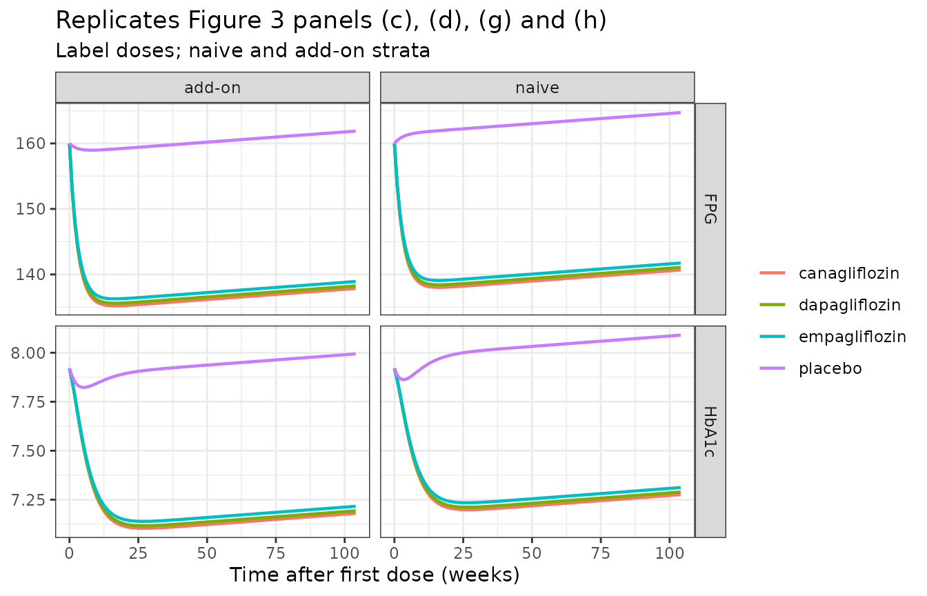

active_summary <- active |>
  dplyr::filter(stratum == "naive") |>
  dplyr::group_by(arm) |>
  dplyr::summarise(
    fpg_ss = FPG[time == 52],
    hba1c_ss = HbA1c[time == 52],
    .groups = "drop"
  ) |>
  dplyr::mutate(
    d_fpg = fpg_ss - 160,
    d_hba1c = hba1c_ss - 7.92
  )

knitr::kable(
  active_summary |>
    dplyr::rename(
      "Arm" = arm, "FPG at week 52" = fpg_ss, "HbA1c at week 52" = hba1c_ss,
      "FPG change from baseline" = d_fpg, "HbA1c change from baseline" = d_hba1c
    ),
  digits = 3,
  caption = "Naive-stratum endpoint change from baseline at week 52, at each drug's label dose."
)

Naive-stratum endpoint change from baseline at week 52, at each drug’s label dose.
Arm	FPG at week 52	HbA1c at week 52	FPG change from baseline	HbA1c change from baseline
canagliflozin	139.057	7.221	-20.943	-0.699
dapagliflozin	139.446	7.234	-20.554	-0.686
empagliflozin	140.120	7.257	-19.880	-0.663
placebo	163.078	8.034	3.078	0.114


drug_rows <- active_summary[active_summary$arm != "placebo", ]

# Each drug must lower both endpoints relative to baseline, and the three must
# land close together (the paper's central claim: same Emax, different EC50, so
# similar efficacy at label doses). Deterministic typical-value solve.
stopifnot(
  all(drug_rows$d_fpg < -15),
  all(drug_rows$d_hba1c < -0.6),
  diff(range(drug_rows$d_fpg)) < 2,
  diff(range(drug_rows$d_hba1c)) < 0.1
)

# The HbA1c reductions must be clinically plausible: SGLT2-inhibitor phase III
# trials report roughly -0.6 to -1.0% total change from baseline at label dose.
stopifnot(all(drug_rows$d_hba1c > -1.2), all(drug_rows$d_hba1c < -0.5))

The FPG onset rate, and why the drug term carries it

onset <- active |>
  dplyr::filter(stratum == "naive", arm == "dapagliflozin") |>
  dplyr::select(time, FPG)

fpg_span <- onset$FPG[onset$time == 0] - min(onset$FPG)
t90 <- min(onset$time[onset$FPG <= onset$FPG[onset$time == 0] - 0.9 * fpg_span])

kfp <- exp(ep_ui$theta[["lkfp"]])
kout <- exp(ep_ui$theta[["lkout"]])

knitr::kable(
  data.frame(
    Quantity = c(
      "Kfp (1/week)", "FPG response half-life (weeks)",
      "Kout (1/week)", "HbA1c turnover half-life (weeks)",
      "Simulated weeks to 90% of the FPG fall"
    ),
    Value = c(kfp, log(2) / kfp, kout, log(2) / kout, t90)
  ),
  digits = 3,
  caption = "Response time constants."
)

Response time constants.
Quantity	Value
Kfp (1/week)	0.340
FPG response half-life (weeks)	2.039
Kout (1/week)	0.200
HbA1c turnover half-life (weeks)	3.466
Simulated weeks to 90% of the FPG fall	7.000


# Yao 2023 Discussion: Kfp of 0.34 /week is "a half-life of 2 weeks", and Kout
# of 0.20 /week is "a half-life of 3.5 weeks". Both are exact arithmetic.
stopifnot(
  abs(log(2) / kfp - 2) < 0.05,
  abs(log(2) / kout - 3.5) < 0.05
)

# The drug-arm FPG fall must be GRADUAL, not an instantaneous step at t = 0.
# Equation 4 as printed omits the (1 - exp(-Kfp*t)) factor and would make it a
# step; Figure 3(c) shows the simulated median leaving the 160 mg/dL baseline
# and reaching plateau at about 3/Kfp = 8.8 weeks. The model reproduces that.
stopifnot(
  abs(onset$FPG[onset$time == 0] - 160) < 1e-8,
  abs(t90 - log(10) / kfp) < 1.5
)

Between-study variability

The four models carry between-study, not between-subject, variability. The band below is therefore the spread of study-arm means a meta-analysis of this size would see, which is what Figure 3’s simulated percentiles represent.

n_studies <- 200

itv_rows <- dplyr::bind_rows(lapply(c("placebo", "dapagliflozin"), function(a) {
  dplyr::bind_cols(
    data.frame(arm = rep(a, n_studies)),
    auc_cols(if (a == "placebo") "none" else a,
             if (a == "placebo") 0 else auc_label[["dapagliflozin"]]),
    strata_cols("naive")[rep(1, n_studies), , drop = FALSE]
  )
}))

itv_ev <- ep_events(itv_rows, seq(0, 104, by = 4))
itv <- rxode2::rxSolve(
  readModelDb("Yao_2023_sglt2_endpoints_mbma"),
  itv_ev, keep = "arm", returnType = "data.frame"
)
#> ℹ parameter labels from comments will be replaced by 'label()'

itv_band <- itv |>
  dplyr::group_by(arm, time) |>
  dplyr::summarise(
    p05 = quantile(HbA1c, 0.05),
    p50 = median(HbA1c),
    p95 = quantile(HbA1c, 0.95),
    .groups = "drop"
  )

ggplot(itv_band, aes(time, p50, colour = arm, fill = arm)) +
  geom_ribbon(aes(ymin = p05, ymax = p95), alpha = 0.2, colour = NA) +
  geom_line(linewidth = 0.8) +
  labs(
    x = "Time after first dose (weeks)", y = "HbA1c (%)", colour = NULL, fill = NULL,
    title = "Between-study spread of study-arm mean HbA1c (naive stratum)",
    subtitle = paste0(n_studies, " simulated study arms; median and 5th-95th percentile")
  ) +
  theme_bw()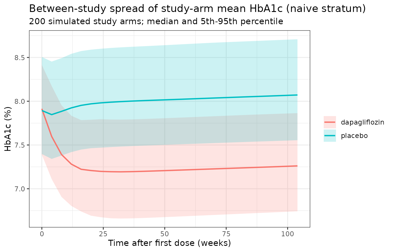

# These are COHORT-derived quantities. rxSetSeed() fixes the draw only for a
# given solver thread count, so the bounds below are deliberately loose enough
# to survive a different cohort while still failing on a mis-transcribed
# parameter (which moves HbA1c by several tenths of a percent).
itv_end <- itv_band[itv_band$time == 104, ]
placebo_end <- itv_end$p50[itv_end$arm == "placebo"]
drug_end <- itv_end$p50[itv_end$arm == "dapagliflozin"]

stopifnot(
  # The drug arm must sit clearly below the placebo arm at the end of follow-up.
  placebo_end - drug_end > 0.4,
  # Both medians must stay inside a physiologically sensible HbA1c range.
  drug_end > 6, placebo_end < 9,
  # The between-study band must be non-degenerate but not implausibly wide.
  all(itv_end$p95 - itv_end$p05 > 0.05),
  all(itv_end$p95 - itv_end$p05 < 3)
)

Assumptions and deviations

Two printed equations reconciled against the paper’s own outputs

Two of the eight printed equations do not reproduce the paper’s own figures as written. Both are transcribed here in the form that does, with the evidence recorded next to the equation in inst/modeldb/specificDrugs/Yao_2023_sglt2_endpoints_mbma.R.

Equation 5 sign (HbA1c placebo response). Printed as HbA1c_placebo = HbA1c_baseline - Phmax * (1 - exp(-Khp*t)) + DIShp*t, while Table 2 reports signed Phmax values (-0.200, +0.0510, -0.230, -0.06 %). Taking both literally double-negates and makes the naive placebo arm rise. The Results text states the opposite (“the estimated Phmax value in HbA1c for naive groups, add-on groups, and mixed groups were -0.20%, -0.23%, and -0.06% decrease from baseline while that of non-naive groups was 0.051% increase from baseline”), and Figure 3(e) shows the simulated placebo median dipping about 0.15% below baseline before disease progression carries it back up. The companion FPG Equation 3 uses + Pfmax with the same signed convention. This model uses + Phmax.
Equation 4 onset (FPG drug effect). Printed as FPG = FPG_placebo + SLOPEfd * dUGEc, which makes the drug effect an instantaneous step at t = 0. The Discussion attributes the onset rate to the drug effect (“The FPG responses in drug effects with a Kfp of 0.34 weeks-1 or a half-life of 2 weeks indicated a 2-week continuous treatment could show a significant decrease in FPG”), yet Kfp appears only in Equation 3. Figure 3 panels (c) and (d) settle it: the simulated median starts at the 160 mg/dL baseline at t = 0 and reaches its plateau at about 9 weeks, which is 3 / Kfp = 8.8 weeks. A step would put the median at the plateau already at t = 0. This model multiplies the drug term by (1 - exp(-Kfp * t)) – the minimal change that reproduces the figure, and algebraically identical to folding SLOPEfd * dUGEc into the Pfmax slot of Equation 3.

Reading of Equation 7

The unsubscripted HbA1c in the elimination term of Equation 7 is taken to be the total of Equation 8 (placebo + drug). That is the literal reading of the symbol and the only one under which the stated initial condition HbA1c_drug(0) = 0 is stationary when there is no drug and no placebo effect; reading it as HbA1c_drug alone drives that state to the HbA1c baseline and doubles the predicted HbA1c.

The dapagliflozin food-effect equation is not printed

Table 1 reports the fed-state coefficient as a bare 0.254 with no covariate equation anywhere in the paper or in Appendix S1. It is applied here as a multiplier, Kt_fed = Kt * 0.254. That is the standard NONMEM encoding for a covariate reported as a bare fraction, it is the only reading that produces the “longer time to maximum concentration” the Discussion describes, and it moves the simulated Tmax from roughly 1 h fasted to roughly 2 h fed, matching the observed dapagliflozin high-fat-meal effect. The alternative reading Kt * (1 - 0.254) changes Tmax by only about a third and would not be a significant covariate at p < 0.005.

Residual-error weighting

Appendix S1 Equation S14 writes the residual model as Y_obs = Y_pred + Y_pred * eps1 * W + eps2 * W with W the square root of the study sample size, so a larger study would carry a larger residual. The usual NONMEM convention for a meta-analysis weight is the reverse (divide by sqrt(N)), and the reported variances are only plausible under one direction for the PK layer and the other for the endpoint layer: the PK proportional SD of 0.676 is 68% at W = 1, implausible for study-arm means unless divided, whereas the FPG additive SD of 0.18 mg/dL is implausibly small unless multiplied. The direction is not resolvable from any on-disk source. The models therefore carry the reported variances back-transformed to SD at W = 1, verbatim, and every validation above uses rxode2::zeroRe() typical-value solves so that no conclusion depends on the weighting. A downstream user simulating a study of N subjects must decide the direction themselves.

Other assumptions

Inter-study, not inter-individual. Table 1 and Table 2 head the variance column “IIV (%)”, but Appendix S1 section 1.2 defines it as inter-study variability. All etas are named eta_study_* and the models simulate study-arm means only.
IIV(%) to omega. Exponential terms use omega^2 = log((IIV/100)^2 + 1); the additive terms on Pfmax and Phmax use omega^2 = ((IIV/100) * |value|)^2, the same reading applied to the sibling T2DM meta-analysis modellib("Li_2015_taspoglutide_mbma").
Apparent PK parameters. The paper fits oral data only and reports no bioavailability term, so CL, Vc, CLD and VT are apparent (CL/F, Vc/F, …).
Canagliflozin clearance. The fitted CL/F of 12.0 L/h is roughly a third of the value implied by the labelled single-dose AUC, so AUC_CANA computed from this model is correspondingly larger than a label-derived AUC. The canagliflozin EC50 of 2310 ng*h/mL is scaled to the same internal exposure, so the pair is self-consistent; an externally derived canagliflozin AUC must not be fed to this endpoint model.
SLOPEfd units. Table 2 prints “mg/dL^2”. For SLOPEfd * dUGEc to have units of mg/dL with dUGEc in g/(mg/dL), the coefficient must be (mg/dL)^2 per g. The numeric value is used as printed.
Not extracted. The external-validation exercise against ertugliflozin (Figure 4) reuses the endpoint model with an ertugliflozin PK/PD model whose parameters the paper does not tabulate, so no ertugliflozin model file is produced. The MPG-corrected variant of the biomarker (Figure S4) was rejected by the authors on objective-function value and is not extracted.

Session information

#> R version 4.6.1 (2026-06-24)
#> Platform: x86_64-pc-linux-gnu
#> Running under: Ubuntu 24.04.4 LTS
#> 
#> Matrix products: default
#> BLAS:   /usr/lib/x86_64-linux-gnu/openblas-pthread/libblas.so.3 
#> LAPACK: /usr/lib/x86_64-linux-gnu/openblas-pthread/libopenblasp-r0.3.26.so;  LAPACK version 3.12.0
#> 
#> locale:
#>  [1] LC_CTYPE=C.UTF-8       LC_NUMERIC=C           LC_TIME=C.UTF-8       
#>  [4] LC_COLLATE=C.UTF-8     LC_MONETARY=C.UTF-8    LC_MESSAGES=C.UTF-8   
#>  [7] LC_PAPER=C.UTF-8       LC_NAME=C              LC_ADDRESS=C          
#> [10] LC_TELEPHONE=C         LC_MEASUREMENT=C.UTF-8 LC_IDENTIFICATION=C   
#> 
#> time zone: UTC
#> tzcode source: system (glibc)
#> 
#> attached base packages:
#> [1] stats     graphics  grDevices utils     datasets  methods   base     
#> 
#> other attached packages:
#> [1] ggplot2_4.0.3         tidyr_1.3.2           dplyr_1.2.1          
#> [4] rxode2_5.1.6          PKNCA_0.12.1          nlmixr2lib_0.3.2.9000
#> 
#> loaded via a namespace (and not attached):
#>  [1] gtable_0.3.6        xfun_0.60           bslib_0.12.0       
#>  [4] lattice_0.22-9      vctrs_0.7.3         tools_4.6.1        
#>  [7] generics_0.1.4      parallel_4.6.1      tibble_3.3.1       
#> [10] symengine_0.2.13    pkgconfig_2.0.3     data.table_1.18.6.1
#> [13] checkmate_2.3.4     RColorBrewer_1.1-3  S7_0.2.2           
#> [16] desc_1.4.3          RcppParallel_6.2.1  lifecycle_1.0.5    
#> [19] compiler_4.6.1      farver_2.1.2        textshaping_1.0.5  
#> [22] fontawesome_0.5.3   htmltools_0.5.9     sys_3.4.3          
#> [25] sass_0.4.10         yaml_2.3.12         pillar_1.11.1      
#> [28] pkgdown_2.2.1       crayon_1.5.3        jquerylib_0.1.4    
#> [31] whisker_0.4.1       openssl_2.4.2       cachem_1.1.0       
#> [34] nlme_3.1-169        tidyselect_1.2.1    digest_0.6.39      
#> [37] lotri_1.0.4         purrr_1.2.2         labeling_0.4.3     
#> [40] rxode2ll_2.0.16     fastmap_1.2.0       grid_4.6.1         
#> [43] cli_3.6.6           dparser_1.3.1-13    magrittr_2.0.5     
#> [46] withr_3.0.3         scales_1.4.0        backports_1.5.1    
#> [49] rmarkdown_2.32      otel_0.2.0          askpass_1.2.1      
#> [52] ragg_1.5.2          memoise_2.0.1       evaluate_1.0.5     
#> [55] knitr_1.52          rex_1.2.2           PreciseSums_0.7    
#> [58] rlang_1.3.0         downlit_0.4.5       Rcpp_1.1.2         
#> [61] glue_1.8.1          xml2_1.6.0          jsonlite_2.0.0     
#> [64] R6_2.6.1            systemfonts_1.3.2   fs_2.1.0