Artesunate + mefloquine in Plasmodium berghei-infected mice (Mim 2026)
Source:vignettes/articles/Mim_2026_mefloquine_artesunate.Rmd
Mim_2026_mefloquine_artesunate.RmdModel and source
Mim 2026 gave Plasmodium berghei-infected Swiss mice a single oral dose of artesunate (AS) 100 mg/kg plus mefloquine (MQ) 55 mg/kg and fitted, in Monolix 2024R1:
- a two-compartment PK model with first-order absorption for each drug (Tables 1 and 2), fitted separately;
- a turnover model of percent parasitemia in which the plasma concentration of each drug inhibits parasite production, the two inhibitions adding (Equation 1, Table 3).
Both parts are packaged in one model,
Mim_2026_mefloquine_artesunate_mouse, with every mefloquine
quantity suffixed _mefloquine and every artesunate quantity
_artesunate. Artesunate monotherapy is simulated by giving
no mefloquine dose.
- Citation: Mim SR, Vieira Santos V, Pereira LC, Pica K, Miranda ALLdS, Quadros HC, Moreira DRM, Azeredo FJ. (2026). Pharmacokinetic and pharmacodynamic modeling of anti-plasmodial drugs mefloquine plus artesunate: insights on translational application. Antimicrob Agents Chemother 70(3):e01717-25. doi:10.1128/aac.01717-25.
- Description: Preclinical (mouse, Plasmodium berghei-infected). Population PK/PD model of oral artesunate plus mefloquine (ASMQ) given as a single gavage dose. Each drug has its own two-compartment PK model with first-order absorption and linear elimination, fitted separately in Monolix (Mim 2026 Tables 1 and 2). The plasma concentrations of both drugs drive one turnover model of percent parasitemia in which each drug inhibits parasite production with an Imax = 1, Hill = 1 function and the two inhibitions add (Equation 1, Table 3). The additive sum is capped at 1 so that production cannot become negative; with the cap the model reproduces the published combination simulations (Figure 4a), whereas the uncapped Equation 1 drives parasitemia below zero within 10 h. Between-animal variability was fixed to a negligible value (sparse destructive sampling) and is carried as fixed etas. Set the mefloquine dose to zero for artesunate monotherapy.
- Article: https://doi.org/10.1128/aac.01717-25
Population
Male and female Swiss mice (6-8 weeks, 18-22 g) were inoculated intraperitoneally with 1e6 erythrocytes parasitised by P. berghei ANKA gfp/luc. Once parasitemia reached 5% or more, the PK animals received the 100/55 mg/kg combination by gavage and were sampled destructively, four per time point, at 0.083-48 h (Methods). The data set held 59 mefloquine and 34 artesunate plasma samples measured by HPLC-DAD. Parasitemia was read by flow cytometry; the treated-group means are in Table S1.
str(readModelDb("Mim_2026_mefloquine_artesunate_mouse")()$population)
#> List of 9
#>  $ species      : chr "mouse (Swiss, Plasmodium berghei ANKA gfp/luc-infected)"
#>  $ n_subjects   : int 44
#>  $ n_studies    : int 1
#>  $ age_range    : chr "6-8 weeks"
#>  $ weight_range : chr "18-22 g"
#>  $ disease_state: chr "Plasmodium berghei blood-stage malaria after intraperitoneal inoculation of 1e6 parasitized erythrocytes; PK an"| __truncated__
#>  $ dose_range   : chr "Single oral (gavage) dose of artesunate 100 mg/kg plus mefloquine 55 mg/kg"
#>  $ regions      : chr "Brazil (Instituto Goncalo Moniz, Fiocruz, Salvador)"
#>  $ notes        : chr "Male and female Swiss mice (proportions not reported). PK by destructive sampling, n = 4 per time point at 0.08"| __truncated__
Source trace
| Parameter / equation | Value | Source location |
|---|---|---|
| Two-compartment PK, first-order absorption, each drug | n/a | Results, Pharmacokinetic model; Figure 5 |
lka_mefloquine |
0.28 1/h | Table 1, Ka |
lcl_mefloquine |
286.01 mL/h/kg | Table 1, CL |
lvc_mefloquine |
4039.63 mL/kg | Table 1, V1 |
lvp_mefloquine |
41817.36 mL/kg | Table 1, second volume row (V2) |
lq_mefloquine |
20636.48 mL/h/kg | Table 1, Q |
propSd_mefloquine |
0.71 | Table 1, proportional error model |
lka_artesunate |
0.6 1/h (fixed) | Table 2, Ka; Methods |
lcl_artesunate |
3285.52 mL/h/kg | Table 2, CL |
lvc_artesunate |
1921.4 mL/kg | Table 2, V1 |
lvp_artesunate |
11342.3 mL/kg (fixed) | Table 2, second volume row (V2) |
lq_artesunate |
19210.83 mL/h/kg | Table 2, Q |
propSd_artesunate |
0.52 | Table 2, proportional error model |
Turnover ODE, additive inhibition, kin = R0 * kout
|
n/a | Equation 1 and its legend |
lrbase |
17.8 % (fixed) | Table 3, R0 |
lkout |
0.08 1/h (fixed) | Table 3, Kout |
lic50_mefloquine |
0.011 ug/mL | Table 3, IC50 (MQ) |
lic50_artesunate |
0.0044 ug/mL | Table 3, IC50 (AS) |
addSd_parasites |
0.52 % | Table 3, constant error model |
| All etas | variance 1e-6 (fixed) | Results (“IIV fixed to a minimal value of 0.001”); Methods |
| Cap of the summed inhibition at 1 | n/a | Not in Equation 1; inferred from Figure 4a (see below) |
Table 3 gives each IC50 in ug/mL and in nM. The molar values follow from the mass values and the free-base molecular weights (mefloquine 378.3 g/mol, artesunate 384.4 g/mol):
ic50_nm <- c(
  mefloquine = 0.011 / 378.3 * 1e6,
  artesunate = 0.0044 / 384.4 * 1e6
)
round(ic50_nm, 2)
#> mefloquine artesunate
#>      29.08      11.45
# Mefloquine reproduces the printed 29.1 nM; artesunate gives 11.4 nM against
# the printed 10.93 nM, a 5% difference consistent with the ug/mL value being
# rounded to two significant figures.
stopifnot(
  abs(ic50_nm[["mefloquine"]] / 29.1 - 1) < 0.01,
  abs(ic50_nm[["artesunate"]] / 10.93 - 1) < 0.06
)
Simulation set-up
mod <- readModelDb("Mim_2026_mefloquine_artesunate_mouse")
mod_typ <- rxode2::zeroRe(mod)
#> ℹ parameter labels from comments will be replaced by 'label()'

obs_times <- sort(unique(c(seq(0, 2, by = 0.05), seq(2.25, 72, by = 0.25))))

regimens <- tibble::tribble(
  ~regimen,                    ~dose_as, ~dose_mq,
  "100 mg/kg AS + 55 mg/kg MQ",     100,       55,
  "25 mg/kg AS + 55 mg/kg MQ",       25,       55,
  "100 mg/kg AS alone",             100,        0,
  "55 mg/kg MQ alone",                0,       55
)

make_events <- function(i, n, obs_cmt = "parasites") {
  r <- regimens[i, ]
  ids <- (i - 1) * n + seq_len(n)
  dose <- dplyr::bind_rows(
    if (r$dose_mq > 0) tibble::tibble(id = ids, time = 0, amt = r$dose_mq, evid = 1, cmt = "depot_mefloquine"),
    if (r$dose_as > 0) tibble::tibble(id = ids, time = 0, amt = r$dose_as, evid = 1, cmt = "depot_artesunate")
  )
  obs <- tidyr::expand_grid(id = ids, time = obs_times) |>
    dplyr::mutate(amt = 0, evid = 0, cmt = obs_cmt)
  dplyr::bind_rows(dose, obs) |>
    dplyr::mutate(regimen = r$regimen) |>
    dplyr::arrange(id, time, dplyr::desc(evid))
}

# One typical-value solve per regimen: a multi-subject solve of a zeroRe()
# model warns that no omega is available.
solve_typical <- function(i) {
  rxode2::rxSolve(mod_typ, events = make_events(i, n = 1), keep = "regimen") |>
    as.data.frame()
}
sim_typ <- dplyr::bind_rows(lapply(seq_len(nrow(regimens)), solve_typical)) |>
  dplyr::mutate(regimen = factor(regimen, levels = regimens$regimen))
#> ℹ omega/sigma items treated as zero: 'etalka_mefloquine', 'etalcl_mefloquine', 'etalvc_mefloquine', 'etalvp_mefloquine', 'etalq_mefloquine', 'etalka_artesunate', 'etalcl_artesunate', 'etalvc_artesunate', 'etalvp_artesunate', 'etalq_artesunate', 'etalrbase', 'etalkout', 'etalic50_mefloquine', 'etalic50_artesunate'
#> ℹ omega/sigma items treated as zero: 'etalka_mefloquine', 'etalcl_mefloquine', 'etalvc_mefloquine', 'etalvp_mefloquine', 'etalq_mefloquine', 'etalka_artesunate', 'etalcl_artesunate', 'etalvc_artesunate', 'etalvp_artesunate', 'etalq_artesunate', 'etalrbase', 'etalkout', 'etalic50_mefloquine', 'etalic50_artesunate'
#> ℹ omega/sigma items treated as zero: 'etalka_mefloquine', 'etalcl_mefloquine', 'etalvc_mefloquine', 'etalvp_mefloquine', 'etalq_mefloquine', 'etalka_artesunate', 'etalcl_artesunate', 'etalvc_artesunate', 'etalvp_artesunate', 'etalq_artesunate', 'etalrbase', 'etalkout', 'etalic50_mefloquine', 'etalic50_artesunate'
#> ℹ omega/sigma items treated as zero: 'etalka_mefloquine', 'etalcl_mefloquine', 'etalvc_mefloquine', 'etalvp_mefloquine', 'etalq_mefloquine', 'etalka_artesunate', 'etalcl_artesunate', 'etalvc_artesunate', 'etalvp_artesunate', 'etalq_artesunate', 'etalrbase', 'etalkout', 'etalic50_mefloquine', 'etalic50_artesunate'
Pharmacokinetics
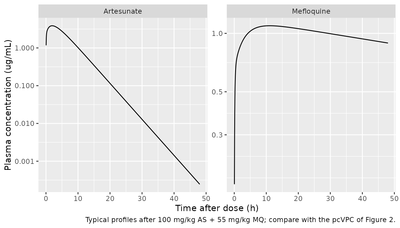
Typical plasma profiles (Figure 2)
sim_typ |>
  dplyr::filter(regimen == "100 mg/kg AS + 55 mg/kg MQ", time > 0, time <= 48) |>
  dplyr::select(time, Mefloquine = Cc_mefloquine, Artesunate = Cc_artesunate) |>
  tidyr::pivot_longer(-time, names_to = "drug", values_to = "conc") |>
  ggplot(aes(time, conc)) +
  geom_line() +
  facet_wrap(~drug, scales = "free_y") +
  scale_y_log10() +
  labs(
    x = "Time after dose (h)", y = "Plasma concentration (ug/mL)",
    caption = "Typical profiles after 100 mg/kg AS + 55 mg/kg MQ; compare with the pcVPC of Figure 2."
  )
PKNCA
The paper reports no NCA table for the mice. The Discussion quotes an observed artesunate Cmax of “approximately 6,500 ng/mL” (6.5 ug/mL), which is the only published exposure value to compare with.
pk_typ <- sim_typ |>
  dplyr::filter(regimen == "100 mg/kg AS + 55 mg/kg MQ") |>
  dplyr::select(time, Mefloquine = Cc_mefloquine, Artesunate = Cc_artesunate) |>
  tidyr::pivot_longer(-time, names_to = "drug", values_to = "Cc") |>
  dplyr::mutate(id = 1L, treatment = "100 mg/kg AS + 55 mg/kg MQ") |>
  dplyr::filter(!is.na(Cc))
dose_typ <- tibble::tibble(
  id = 1L, time = 0, treatment = "100 mg/kg AS + 55 mg/kg MQ",
  drug = c("Mefloquine", "Artesunate"), amt = c(55, 100)
)

nca_typ <- PKNCA::pk.nca(PKNCA::PKNCAdata(
  PKNCA::PKNCAconc(pk_typ, Cc ~ time | treatment + drug + id),
  PKNCA::PKNCAdose(dose_typ, amt ~ time | treatment + drug + id, route = "extravascular"),
  intervals = data.frame(
    start = 0, end = 72, cmax = TRUE, tmax = TRUE, auclast = TRUE, half.life = TRUE
  )
))
nca_df <- as.data.frame(nca_typ)
nca_df |>
  dplyr::filter(PPTESTCD %in% c("cmax", "tmax", "auclast", "half.life")) |>
  dplyr::select(drug, PPTESTCD, PPORRES) |>
  tidyr::pivot_wider(names_from = PPTESTCD, values_from = PPORRES) |>
  dplyr::rename(
    "Drug" = drug, "Cmax (ug/mL)" = cmax, "Tmax (h)" = tmax,
    "AUC0-72 (ug*h/mL)" = auclast, "Terminal t1/2 (h)" = half.life
  ) |>
knitr::kable(digits = 3, caption = "NCA of the typical profiles after 100 mg/kg AS + 55 mg/kg MQ.")| Drug | AUC0-72 (ug*h/mL) | Cmax (ug/mL) | Tmax (h) | Terminal t1/2 (h) |
|---|---|---|---|---|
| Artesunate | 30.427 | 3.868 | 1.95 | 3.170 |
| Mefloquine | 67.601 | 1.095 | 11.00 | 113.208 |
cmp <- nlmixr2lib::ncaComparisonTable(
  simulated = PKNCA::pk.nca(PKNCA::PKNCAdata(
    PKNCA::PKNCAconc(dplyr::filter(pk_typ, drug == "Artesunate"), Cc ~ time | treatment + id),
    PKNCA::PKNCAdose(dplyr::filter(dose_typ, drug == "Artesunate"), amt ~ time | treatment + id,
                     route = "extravascular"),
    intervals = data.frame(start = 0, end = 72, cmax = TRUE)
  )),
  reference = tibble::tibble(treatment = "100 mg/kg AS + 55 mg/kg MQ", cmax = 6.5),
  by = "treatment",
  units = c(cmax = "ug/mL"),
  tolerance_pct = 20
)
knitr::kable(cmp, caption = "Typical artesunate Cmax vs. the observed value quoted in the Discussion. * differs by >20%.")| NCA parameter | treatment | Reference | Simulated | % diff |
|---|---|---|---|---|
| Cmax (ug/mL) | 100 mg/kg AS + 55 mg/kg MQ | 6.5 | 3.87 | -40.5%* |
cmax_as <- nca_df$PPORRES[nca_df$drug == "Artesunate" & nca_df$PPTESTCD == "cmax"]
cmax_mq <- nca_df$PPORRES[nca_df$drug == "Mefloquine" & nca_df$PPTESTCD == "cmax"]
stopifnot(
  # The typical artesunate peak (about 3.9 ug/mL at 2 h) is below the observed
  # 6.5 ug/mL; see Assumptions. It must still be within a factor of two, which
  # a unit slip (1000-fold) or a swapped V1/V2 would not be.
  cmax_as > 6.5 / 2, cmax_as < 6.5,
  # Mefloquine stays in the 0.75-24 ug/mL calibrated range of the assay.
  cmax_mq > 0.75, cmax_mq < 24
)
The typical artesunate Cmax (3.87 ug/mL) is about 40% below the “approximately 6,500 ng/mL” quoted in the Discussion. That figure is an observed peak from four destructively sampled animals per time point, and the artesunate residual error is large (proportional SD 0.52), so a typical-value prediction below the highest observed mean is expected rather than a sign of a transcription error.
Pharmacodynamics
Equation 1 as printed, and the cap
Both drugs are far above their IC50 within minutes of the dose (mefloquine about 1 ug/mL against 0.011 ug/mL, artesunate about 3 ug/mL against 0.0044 ug/mL), so each inhibition term is close to 1 and their printed sum is close to 2. Equation 1 then makes parasite production negative and drives parasitemia below zero within about 9 h. The packaged model caps the summed inhibition at 1; the comparison below shows that only the capped form reproduces Figure 4a.
mod_uncapped <- mod_typ |>
  rxode2::model(inh_total <- inh_mefloquine + inh_artesunate)
ev_combo <- make_events(1, n = 1)
sim_uncapped <- rxode2::rxSolve(mod_uncapped, events = ev_combo) |> as.data.frame()
#> ℹ omega/sigma items treated as zero: 'etalka_mefloquine', 'etalcl_mefloquine', 'etalvc_mefloquine', 'etalvp_mefloquine', 'etalq_mefloquine', 'etalka_artesunate', 'etalcl_artesunate', 'etalvc_artesunate', 'etalvp_artesunate', 'etalq_artesunate', 'etalrbase', 'etalkout', 'etalic50_mefloquine', 'etalic50_artesunate'

fig4a <- tibble::tribble(
  ~time, ~figure,
      8,     9.5,
     24,     2.7,
     36,     1.0,
     48,     0.5
)
chk4a <- sim_typ |>
  dplyr::filter(regimen == "100 mg/kg AS + 55 mg/kg MQ", time %in% fig4a$time) |>
  dplyr::select(time, capped = parasites) |>
  dplyr::left_join(
    sim_uncapped |> dplyr::filter(time %in% fig4a$time) |> dplyr::select(time, uncapped = parasites),
    by = "time"
  ) |>
  dplyr::left_join(fig4a, by = "time")
chk4a |>
  dplyr::rename(
    "Time (h)" = time, "Capped (packaged)" = capped,
    "Equation 1 as printed" = uncapped, "Figure 4a median" = figure
  ) |>
knitr::kable(digits = 2, caption = "Typical parasitemia (%) after 100 mg/kg AS + 55 mg/kg MQ.")| Time (h) | Capped (packaged) | Equation 1 as printed | Figure 4a median |
|---|---|---|---|
| 8 | 9.39 | 1.09 | 9.5 |
| 24 | 2.61 | -12.00 | 2.7 |
| 36 | 1.00 | -11.96 | 1.0 |
| 48 | 0.38 | -6.30 | 0.5 |
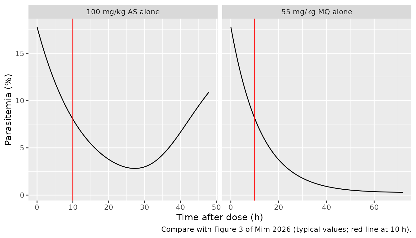
Figure 3 – each drug’s contribution
sim_typ |>
  dplyr::filter(regimen %in% c("55 mg/kg MQ alone", "100 mg/kg AS alone")) |>
  dplyr::filter((regimen == "55 mg/kg MQ alone" & time <= 72) |
                  (regimen == "100 mg/kg AS alone" & time <= 48)) |>
  ggplot(aes(time, parasites)) +
  geom_line() +
  geom_vline(xintercept = 10, colour = "red") +
  facet_wrap(~regimen, scales = "free_x") +
  labs(
    x = "Time after dose (h)", y = "Parasitemia (%)",
    caption = "Compare with Figure 3 of Mim 2026 (typical values; red line at 10 h)."
  )
r10 <- sim_typ |>
  dplyr::filter(time == 10, regimen %in% c("55 mg/kg MQ alone", "100 mg/kg AS alone")) |>
  dplyr::select(regimen, parasites)
r10 |>
  dplyr::rename("Regimen" = regimen, "Parasitemia at 10 h (%)" = parasites) |>
knitr::kable(digits = 2, caption = "Typical parasitemia (%) 10 h after each drug alone.")| Regimen | Parasitemia at 10 h (%) |
|---|---|
| 100 mg/kg AS alone | 8.02 |
| 55 mg/kg MQ alone | 8.11 |
as_alone <- dplyr::filter(sim_typ, regimen == "100 mg/kg AS alone", time <= 48)
stopifnot(
  # Results: artesunate reduces parasitemia to about 8% at 10 h.
  abs(r10$parasites[r10$regimen == "100 mg/kg AS alone"] - 8) < 0.5,
  # Artesunate alone reaches a minimum and rebounds before 48 h.
  as_alone$parasites[as_alone$time == 48] > min(as_alone$parasites) + 2
)
The artesunate panel matches Figure 3 (right) at 10 h. The simulated minimum, about 2.8% at 27.25 h, is earlier and higher than the roughly 1.7% at 35 h in the figure. The mefloquine panel does not match Figure 3 (left): the figure falls to about 11.6% at 10 h and 1% at 72 h, a decline at roughly half of Kout, whereas with Kout = 0.08 1/h and mefloquine far above its IC50 the model gives about 8.1% at 10 h. No parameter set in Tables 1-3 produces the slower curve; see Assumptions.
Figure 4 – dosing regimens
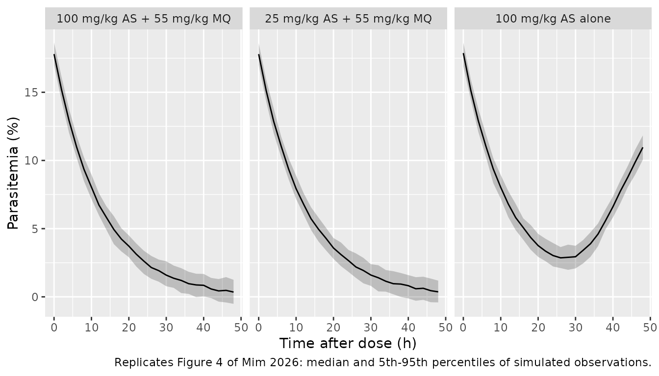
Figure 4 shows 1,000 simulated animals per regimen. With all IIV fixed to a negligible value the band comes from the residual error alone; 200 animals per regimen are simulated here.
rxode2::rxSetSeed(20260212)
ev_vpc <- dplyr::bind_rows(lapply(1:3, make_events, n = 200)) |>
  dplyr::filter(evid == 1 | time %in% seq(0, 48, by = 2))
sim_vpc <- rxode2::rxSolve(mod, events = ev_vpc, keep = "regimen") |>
  as.data.frame() |>
  dplyr::mutate(regimen = factor(regimen, levels = regimens$regimen[1:3]))
#> ℹ parameter labels from comments will be replaced by 'label()'

vpc_sum <- sim_vpc |>
  dplyr::group_by(regimen, time) |>
  dplyr::summarise(
    Q05 = quantile(sim, 0.05), Q50 = median(sim), Q95 = quantile(sim, 0.95),
    .groups = "drop"
  )
ggplot(vpc_sum, aes(time, Q50)) +
  geom_ribbon(aes(ymin = Q05, ymax = Q95), alpha = 0.25) +
  geom_line() +
  facet_wrap(~regimen) +
  labs(
    x = "Time after dose (h)", y = "Parasitemia (%)",
    caption = "Replicates Figure 4 of Mim 2026: median and 5th-95th percentiles of simulated observations."
  )
med24 <- vpc_sum |> dplyr::filter(time == 24)
stopifnot(
  # Results: both combination regimens give the same profile.
  abs(med24$Q50[med24$regimen == "100 mg/kg AS + 55 mg/kg MQ"] -
        med24$Q50[med24$regimen == "25 mg/kg AS + 55 mg/kg MQ"]) < 0.5,
  # Residual-only band: the 90% interval is 2 * 1.645 * 0.52 = 1.7 points
  # wide. Asserted on the median over time points, since each width is a
  # quantile estimate from 200 draws.
  abs(median((vpc_sum$Q95 - vpc_sum$Q05) / (2 * 1.645 * 0.52)) - 1) < 0.1
)
Figure 4b (artesunate alone) starts at about 22.5%, not 17.8%; the paper does not say which baseline that panel used. Expressed as a fraction of the starting value, the figure and the typical simulation agree:
fig4b <- tibble::tribble(
  ~time, ~figure,
      0,    22.5,
      8,    12.0,
     24,     4.0,
     36,     6.5,
     48,    14.0
) |>
  dplyr::mutate(figure_frac = figure / 22.5)
chk4b <- sim_typ |>
  dplyr::filter(regimen == "100 mg/kg AS alone", time %in% fig4b$time) |>
  dplyr::transmute(time, model_frac = parasites / 17.8) |>
  dplyr::left_join(fig4b, by = "time")
chk4b |>
  dplyr::select(time, figure_frac, model_frac) |>
  dplyr::rename(
    "Time (h)" = time, "Figure 4b / 22.5%" = figure_frac, "Model / 17.8%" = model_frac
  ) |>
knitr::kable(digits = 3, caption = "Artesunate monotherapy, parasitemia relative to its starting value.")| Time (h) | Figure 4b / 22.5% | Model / 17.8% |
|---|---|---|
| 0 | 1.000 | 1.000 |
| 8 | 0.533 | 0.528 |
| 24 | 0.178 | 0.170 |
| 36 | 0.289 | 0.262 |
| 48 | 0.622 | 0.613 |
The Results text quotes a 78% decline at 24 h and a rebound to about 50% of baseline at 48 h; the model gives 83% and 61%, which is also what Figure 4b shows (82% and 62%).
Observed parasitemia (Table S1)
Table S1, experiment 2, lists the mean parasitemia of the treated groups after the same doses. The paper does not say which parasitemia data the PD model was fitted to, and the model does not track these means closely: the observed means stay near baseline for 24 h (14.5% for the combination) and fall only by 36-48 h, whereas the typical model is already at 2.6% by 24 h. Both reach about 1% by 48 h with the combination, and both show artesunate monotherapy leaving parasitemia well above the combination at 48 h.
s1 <- tibble::tribble(
  ~regimen,                     ~time, ~observed,
  "100 mg/kg AS + 55 mg/kg MQ",     0,    17.4,
  "100 mg/kg AS + 55 mg/kg MQ",     8,    15.3,
  "100 mg/kg AS + 55 mg/kg MQ",    24,    14.5,
  "100 mg/kg AS + 55 mg/kg MQ",    36,     4.0,
  "100 mg/kg AS + 55 mg/kg MQ",    48,     1.12,
  "100 mg/kg AS alone",             0,    20,
  "100 mg/kg AS alone",             8,    15.6,
  "100 mg/kg AS alone",            24,    14.2,
  "100 mg/kg AS alone",            36,     7.6,
  "100 mg/kg AS alone",            48,     8.2
)
sim_typ |>
  dplyr::filter(time %in% s1$time, regimen %in% s1$regimen) |>
  dplyr::transmute(regimen = as.character(regimen), time, typical = parasites) |>
  dplyr::inner_join(s1, by = c("regimen", "time")) |>
  dplyr::rename(
    "Regimen" = regimen, "Time (h)" = time,
    "Typical model (%)" = typical, "Table S1 mean (%)" = observed
  ) |>
knitr::kable(digits = 2, caption = "Typical model vs. Table S1 (experiment 2) mean parasitemia.")| Regimen | Time (h) | Typical model (%) | Table S1 mean (%) |
|---|---|---|---|
| 100 mg/kg AS + 55 mg/kg MQ | 0 | 17.80 | 17.40 |
| 100 mg/kg AS + 55 mg/kg MQ | 8 | 9.39 | 15.30 |
| 100 mg/kg AS + 55 mg/kg MQ | 24 | 2.61 | 14.50 |
| 100 mg/kg AS + 55 mg/kg MQ | 36 | 1.00 | 4.00 |
| 100 mg/kg AS + 55 mg/kg MQ | 48 | 0.38 | 1.12 |
| 100 mg/kg AS alone | 0 | 17.80 | 20.00 |
| 100 mg/kg AS alone | 8 | 9.40 | 15.60 |
| 100 mg/kg AS alone | 24 | 3.03 | 14.20 |
| 100 mg/kg AS alone | 36 | 4.66 | 7.60 |
| 100 mg/kg AS alone | 48 | 10.92 | 8.20 |
Assumptions and deviations
-
Cap on the summed inhibition. Equation 1 adds the
two Imax = 1 inhibition terms. Because both drugs are far above their
IC50 after the dose, the sum approaches 2, parasite production becomes
negative and parasitemia falls below zero within about 9 h. The
published combination simulations (Figure 4a) instead fall exactly as
exp(-Kout t) from 17.8%, which is what production fully switched off – a
total inhibition of 1 – gives. The model therefore uses
min(1, I_MQ + I_AS). A Bliss-independence form,1 - (1 - I_MQ)(1 - I_AS), gives the same predictions to within 0.1 percentage points here, since one drug alone already saturates; the cap was chosen because it keeps the printed additive form wherever the sum is below 1. - Figure 3 (left). The mefloquine-only curve in Figure 3 declines at about half of Kout (about 11.6% at 10 h, 1% at 72 h). The model with Table 3 parameters cannot produce that slope while mefloquine is above its IC50; the model was not altered to match it.
- Figure 4b baseline. The artesunate-alone panel starts at about 22.5%; the comparison above uses the fraction of the starting value.
- Mefloquine Ka. Methods says the absorption rate constants were “fixed at 0.31 h-1 for mefloquine and 0.6 h-1 for artesunate”. Table 1 reports the mefloquine Ka as 0.28 1/h with an RSE of 24.4% and a confidence interval, and the Discussion quotes 0.28 1/h as the estimate, so the model uses 0.28 as an estimated value; 0.31 is read as the initial value.
- Units. Table 1 and Table 2 give volumes in mL/kg and clearances in mL/h/kg; the model uses L/kg and L/h/kg with doses in mg/kg, so concentrations are mg/L = ug/mL, the unit of the Table 3 IC50 values.
- Volume labels. Both tables label the second volume “Volume of central compartment, V2”; it is the peripheral volume.
- Between-animal variability. The Results state IIV was “fixed to a minimal value of 0.001”. Monolix parameterises omega as a standard deviation, so each eta is given a fixed variance of 1e-6. The paper does not name the parameters that carry it; every parameter has one, the Monolix default. Reading 0.001 as a variance instead changes nothing visible.
- Residual error on parasitemia. Table 3 labels the PD residual a “constant error model” of 0.52 and the Results text says additive; it is taken as an additive SD of 0.52 percentage points.
- Sequential fit. The PD model took the individual PK parameters as fixed inputs; with negligible IIV these are the typical values in the model.
- Not reproduced. The prediction-corrected VPCs of Figure 2 need the observed concentrations, which are not published.
- No erratum or correction notice was found for this article (checked 2026-11-12).