Model and source
mod <- readModelDb("Lam_2025_ondansetron")
ui <- rxode2::rxode(mod)
#> ℹ parameter labels from comments will be replaced by 'label()'- Citation: Lam K, Mondick JT, Peltz G, Wu M, Kraft WK. Bayesian Population Pharmacokinetic Modeling of Ondansetron for Neonatal Opioid Withdrawal Syndrome. Clin Transl Sci. 2025;18(2):e70147. doi:10.1111/cts.70147
- Article: https://doi.org/10.1111/cts.70147
- Supplement (Appendix S1, NONMEM control stream of the final model): https://doi.org/10.1111/cts.70147
Lam 2025 characterises ondansetron disposition in neonates with
neonatal opioid withdrawal syndrome (NOWS). Because the neonatal PK data
are sparse (109 plasma samples from 36 neonates, median 3 samples per
neonate), the authors did not fit a de novo model. Instead they updated
a published two-compartment intravenous ondansetron model in infants
aged 1-48 months (the “infant reference model”) with Metropolis-Hastings
MCMC in NONMEM (METHOD=BAYES), supplying log-scale normal
priors for CL, V, V2 and Q that were computed from the reference model
at the cohort median birth weight and postmenstrual age, and a weakly
informative prior for the previously uncharacterised oral absorption
rate constant KA.
The key finding is a much slower absorption rate in neonates (KA = 0.19 /h, i.e. an apparent absorption half-life of about 3.6 h) than the adult assumption used in the pre-trial simulations.
What the final model does and does not include
The paper reports a model-selection exercise (Table 2) that compared
a covariate model (allometric scaling plus a clearance-maturation term
applied at the individual level) against a model with no
individual-level covariate effects, using PSIS-LOO cross-validation. The
model without covariate effects was selected: the
covariate model underpredicted individual concentrations while
performing similarly on individual fits and individual posterior
predictive checks (Results 3.1). The Appendix S1 $PK block
of the final run confirms this - it is CL=EXP(MU_1+ETA(1)),
V=EXP(XMU2), V2=EXP(XMU3),
CLD=EXP(XMU4), KA=EXP(XMU5), with no weight or
age terms.
Allometric scaling and clearance maturation therefore enter the analysis only through the priors, evaluated once at the cohort median birth weight (3.19 kg) and median postmenstrual age (39 1/7 weeks).
The final model therefore has no covariate effect on any
structural parameter. It does read exactly one covariate, and
not as a parameter effect: the mother’s plasma concentration at
delivery, which sets the neonate’s central-compartment initial condition
(A_0(2) = C0 * S2).
data.frame(
  Covariate = names(ui$meta$covariateData),
  Units = vapply(ui$meta$covariateData, function(x) x$units, character(1)),
  Role = "Initial condition on `central` at t = 0 (transplacental transfer)",
  `Source column` = vapply(ui$meta$covariateData, function(x) x$source_name,
                           character(1)),
  row.names = NULL, check.names = FALSE
) |>
knitr::kable(caption = "The only covariate the Lam 2025 final model reads.")| Covariate | Units | Role | Source column |
|---|---|---|---|
| CP0_MAT_NGML | ng/mL | Initial condition on central at t = 0
(transplacental transfer) |
C0 (Appendix S1 $INPUT), ng/mL |
Every demographic the paper screened but did not retain is recorded
in the model’s covariatesDataExcluded metadata for
provenance.
data.frame(
  Covariate = names(ui$meta$covariatesDataExcluded),
  Units = vapply(ui$meta$covariatesDataExcluded, function(x) x$units, character(1)),
  Role = c(
    "Prior only (allometric normalisation to 10.4 kg; prior evaluated at 3.19 kg)",
    "Prior only (clearance-maturation function; prior evaluated at 39 1/7 weeks)",
    "Screened and rejected (higher ELPD but diagnostic misspecification)",
    "Exposure-response figure stratifier only",
    "Exposure-response figure stratifier only"
  ),
  row.names = NULL
) |>
knitr::kable(caption = "Demographics screened by Lam 2025 but not retained in the final model.")| Covariate | Units | Role |
|---|---|---|
| WT_BIRTH | kg | Prior only (allometric normalisation to 10.4 kg; prior evaluated at 3.19 kg) |
| PAGE | months | Prior only (clearance-maturation function; prior evaluated at 39 1/7 weeks) |
| PNA | months | Screened and rejected (higher ELPD but diagnostic misspecification) |
| GA | weeks | Exposure-response figure stratifier only |
| SEXF | (binary) | Exposure-response figure stratifier only |
Population
The analysis cohort is 36 neonates with in-utero opioid exposure enrolled in a substudy of NCT01965704, a double-blind, placebo-controlled, multicenter trial in 98 mother/neonate dyads (Table 1). Mean (SD) gestational age at birth was 38.6 (1.1) weeks, birth weight 3.1 (0.4) kg, and length at birth 49.7 (2.7) cm; the cohort was 18 male / 18 female. The median (min, max) number of neonatal ondansetron doses received was 2 (1, 5) and the median number of plasma samples per neonate was 3 (1, 5). The cohort median birth weight and postmenstrual age used to build the informative priors were 3.19 kg and 39 1/7 weeks (Table 2 footnote).
Mothers randomised to ondansetron received a single 8 mg intravenous dose within 4 h of delivery, repeated once if delivery had not occurred within 4 h (median 1, max 2 doses). Neonates received ondansetron 0.07 mg/kg orally once every 24 h starting on the day of birth, up to five doses, with the first dose given 4-8 h after delivery; the mean (SD) neonatal dose was 0.21 (0.03) mg. Maternal plasma ondansetron concentration at delivery was 28.2 (23.5) ng/mL across 29 maternal samples.
More than half of the neonates had measurable pre-dose ondansetron
from transplacental transfer. Lam 2025 handled this by initialising the
neonatal central compartment to the observed maternal concentration
(Appendix S1 $PK: A_0(2) = C0 * S2, with
S2 = V/1000); the umbilical cord was not carried as an
intermediate compartment.
The same information is available programmatically via
readModelDb("Lam_2025_ondansetron")()$population.
Source trace
The per-parameter origin is recorded as an in-file comment next to
each ini() entry in
inst/modeldb/specificDrugs/Lam_2025_ondansetron.R. The
table below collects them in one place for review.
| Equation / parameter | Value | Source location |
|---|---|---|
lka (KA) |
0.19 /h | Table 3, KA row, posterior median (95% CDI 0.15, 0.23) |
lcl (CL) |
0.58 L/h | Table 3, CL row, posterior median (95% CDI 0.51, 0.67) |
lvc (V) |
0.29 L | Table 3, V row, posterior median (95% CDI 0.26, 0.32) |
lvp (V2) |
0.91 L | Table 3, V2 row, posterior median (95% CDI 0.75, 1.11) |
lq (Q) |
6.15 L/h | Table 3, Q row, posterior median (95% CDI 5.63, 6.74) |
lfdepot (F) |
0.62, fixed | Table 3, F row 0.62 (FIXED); Methods 2.2
“Bioavailability (F) was fixed to 0.62 for all model runs” |
etalcl |
0.54 (log-scale variance) | Table 3, “Interindividual Variability (% CV): CL” row, posterior median 0.54 (84.2% CV; 95% CDI 0.32, 0.92) |
addSd |
8.99 ng/mL | Table 3, “Residual error: Additive error (SD)” row, posterior median 80.9 (95% CDI 59.3, 114.6); table note “SD of sigma = sqrt(posterior median)” |
d/dt(depot) = -ka * depot |
n/a | Appendix S1 $DES: K12=KA,
DADT(1)=-K12*A(1)
|
d/dt(central) = ka*depot - kel*central - k12*central + k21*peripheral1 |
n/a | Appendix S1 $DES: K20=CL/V,
K23=CLD/V, K32=CLD/V2,
DADT(2)=K12*A(1)-K20*A(2)-K23*A(2)+K32*A(3)
|
d/dt(peripheral1) = k12*central - k21*peripheral1 |
n/a | Appendix S1 $DES:
DADT(3)=K23*A(2)-K32*A(3)
|
Cc = 1000 * central / vc |
n/a | Appendix S1 $PK: S2=V/1000 (dose in mg, V
in L, concentration in ng/mL) |
Cc ~ add(addSd) |
n/a | Methods 2.2, Y_ij = Yhat_ij + eps_ij; Appendix S1
$ERROR: Y = F + ERR(1)
|
central(0) = CP0_MAT_NGML * vc / 1000 |
n/a | Appendix S1 $PK: A_0(2) = C0 * S2 with
S2 = V/1000; Results 3.1 (“initializing the neonatal
central compartment to the observed maternal concentrations”) |
CP0_MAT_NGML cohort distribution |
28.2 (23.5) ng/mL, 29 samples | Table 1, “Maternal plasma ondansetron concentration (ng/mL)” |
| beta_CL = 0.76, T_CL = 3.82 months (prior only) | fixed | Table 3 rows “B CL” and “T CL”; Methods 2.2.1 maturation function |
| Allometric exponents 0.75 (CL, Q) / 1 (V, V2), reference weight 10.4 kg (prior only) | fixed | Methods 2.2.1,
P = theta_P * (WT_i / 10.4)^theta_allo
|
Virtual cohort
Original observed data are not publicly available. The cohorts below are virtual populations whose demographics and dosing follow the published trial description (Table 1, Methods 2.1). Two cohort families are simulated:
- A characterisation arm - a single oral 0.07 mg/kg dose with no maternal transfer and dense sampling, used for a clean non-compartmental characterisation of the model (Cmax, Tmax, AUC0-inf, terminal half-life).
-
Trial-replication arms - neonates receiving 1, 2, 3
or 5 oral doses q24h with transplacental maternal transfer, integrated
from birth to 75 h after the last dose (the paper’s
tl), used to reproduce the cumulative AUC0-tl and Cmax distributions underlying Figures 3 and 4.
set.seed(20250211)

n_per_arm <- 120L
first_dose_time <- 6      # h; the trial gave the first neonatal dose 4-8 h after delivery
tau <- 24                 # h; q24h dosing
tl_lag <- 75              # h; the paper integrates to 75 h after the last dose
dose_per_kg <- 0.07       # mg/kg

# Pull the fixed effects straight out of the model so the vignette can never
# drift from the packaged ini() values.
theta_val <- function(nm) {
  d <- ui$iniDf
  v <- d$est[!is.na(d$ntheta) & d$name == nm]
  stopifnot(length(v) == 1L)
  unname(v)
}

# Typical central volume, used to convert the maternal plasma concentration
# into the amount that initialises the neonatal central compartment
# (Appendix S1: A_0(2) = C0 * S2 with S2 = V/1000). The model has no IIV on V,
# so this is exact for every subject.
vc_typ <- exp(theta_val("lvc"))
f_bioav <- exp(theta_val("lfdepot"))
c(vc_L = vc_typ, F = f_bioav)
#> vc_L    F
#> 0.29 0.62

rtnorm <- function(n, mean, sd, lower = -Inf, upper = Inf) {
  out <- stats::rnorm(n, mean, sd)
  bad <- out < lower | out > upper
  while (any(bad)) {
    out[bad] <- stats::rnorm(sum(bad), mean, sd)
    bad <- out < lower | out > upper
  }
  out
}

# Observation grid: fine near time 0 (the maternal-transfer bolus redistributes
# with a distribution half-life of a couple of minutes), fine after each oral
# dose (to resolve Cmax), and hourly out to tl.
make_grid <- function(dose_times, tl) {
  sort(unique(c(
    seq(0, 0.6, by = 0.01),
    seq(0.6, 4, by = 0.05),
    unlist(lapply(dose_times, function(d) d + seq(0, 12, by = 0.25))),
    seq(0, tl, by = 1),
    tl
  ))) |>
    (\(x) x[x <= tl])()
}

make_trial_arm <- function(n_doses, n, id_offset) {
  dose_times <- first_dose_time + tau * seq_len(n_doses) - tau
  tl <- max(dose_times) + tl_lag
  grid <- make_grid(dose_times, tl)

  subj <- tibble(
    id = id_offset + seq_len(n),
    WT_BIRTH = rtnorm(n, 3.1, 0.4, lower = 2.0, upper = 4.6),
    CP0_MAT_NGML = rtnorm(n, 28.2, 23.5, lower = 0, upper = 120),
    arm = paste0(n_doses, if (n_doses == 1) " dose" else " doses"),
    n_doses = n_doses
  )

  oral <- subj |>
    tidyr::crossing(time = dose_times) |>
    mutate(evid = 1L, cmt = "depot", amt = dose_per_kg * WT_BIRTH)

  obs <- subj |>
    tidyr::crossing(time = grid) |>
    mutate(evid = 0L, cmt = "central", amt = NA_real_)

  bind_rows(oral, obs) |>
    arrange(id, time, desc(evid))
}

trial_events <- bind_rows(
  make_trial_arm(1L, n_per_arm, id_offset =   0L),
  make_trial_arm(2L, n_per_arm, id_offset = 200L),
  make_trial_arm(3L, n_per_arm, id_offset = 400L),
  make_trial_arm(5L, n_per_arm, id_offset = 600L)
)
stopifnot(!anyDuplicated(unique(trial_events[, c("id", "time", "evid")])))

# Characterisation arm: single oral dose, no maternal transfer, dense grid.
# CP0_MAT_NGML = 0 is the "born with no drug on board" case, so the profile
# below is the contribution of the oral dose alone.
char_subj <- tibble(
  id = 1000L + seq_len(n_per_arm),
  WT_BIRTH = rtnorm(n_per_arm, 3.1, 0.4, lower = 2.0, upper = 4.6),
  CP0_MAT_NGML = 0,
  arm = "single dose (characterisation)"
)
char_events <- bind_rows(
  char_subj |> mutate(time = 0, evid = 1L, cmt = "depot",
                      amt = dose_per_kg * WT_BIRTH),
  char_subj |>
    tidyr::crossing(time = sort(unique(c(seq(0, 12, by = 0.1),
                                         seq(12, 48, by = 0.5))))) |>
    mutate(evid = 0L, cmt = "central", amt = NA_real_)
) |>
  arrange(id, time, desc(evid))

c(trial_rows = nrow(trial_events), char_rows = nrow(char_events))
#> trial_rows  char_rows
#>     168360      23280
Simulation
useLinCmt = FALSE keeps rxode2 from auto-converting the
explicit three-state ODE system into an analytic linCmt()
solution.
The tightened solver tolerances are load-bearing rather than
cosmetic. This model is stiff (k12 = q/vc is about 21 /h
against ka = 0.19 /h) and the 84% CV on CL puts a few
subjects at CL near 5 L/h, i.e. kel near 19 /h. The paper’s
integration window runs to 75 h past the last dose, by which point those
subjects’ concentrations are about 1e-9 of their Cmax. At rxode2’s
default atol = 1e-8 that tail is below the absolute
tolerance and a handful of records come back very slightly negative
(about -5e-5 ng/mL); PKNCA then returns NA for those
subjects, and a single NA silently propagates into the
arm-level median(). Tightening to atol = 1e-12
removes every negative record across the whole cohort, and the
assertions below fail loudly rather than let a future solver change
reintroduce the problem quietly.
sim_trial <- rxode2::rxSolve(
  mod, events = trial_events,
  keep = c("arm", "n_doses", "WT_BIRTH", "CP0_MAT_NGML"),
  useLinCmt = FALSE, atol = 1e-12, rtol = 1e-10
) |>
  as.data.frame()
#> ℹ parameter labels from comments will be replaced by 'label()'

sim_char <- rxode2::rxSolve(
  mod, events = char_events,
  keep = c("arm", "WT_BIRTH", "CP0_MAT_NGML"),
  useLinCmt = FALSE, atol = 1e-12, rtol = 1e-10
) |>
  as.data.frame()

# rxSolve silently drops subjects when an event table is malformed; assert the
# subject count survived the solve.
stopifnot(
  dplyr::n_distinct(sim_trial$id) == 4L * n_per_arm,
  dplyr::n_distinct(sim_char$id) == n_per_arm
)

# No negative or missing concentrations anywhere: a negative deep-tail record
# is the signature of the tolerance problem described above, and PKNCA turns
# it into a silent NA.
stopifnot(
  !anyNA(sim_trial$Cc), !anyNA(sim_char$Cc),
  min(sim_trial$Cc) >= 0, min(sim_char$Cc) >= 0
)
c(min_Cc_trial = min(sim_trial$Cc), min_Cc_char = min(sim_char$Cc))
#> min_Cc_trial  min_Cc_char
#> 2.516079e-07 0.000000e+00
The maternal-transfer initial condition must be visible in the very
first observation: because the model sets
central(0) <- CP0_MAT_NGML * vc / 1000 and reports
Cc <- 1000 * central / vc, the two conversions cancel
and Cc at time 0 must equal the subject’s maternal
concentration exactly. This is a direct per-subject test of the
A_0(2) = C0 * S2 line in the paper’s $PK
block, and it fails loudly if the covariate is dropped or the unit
conversion is wrong in either direction.
t0 <- sim_trial |> filter(time == 0)
max_abs_err <- max(abs(t0$Cc - t0$CP0_MAT_NGML))
c(subjects_checked = nrow(t0), max_abs_err = max_abs_err)
#> subjects_checked      max_abs_err
#>     4.800000e+02     1.421085e-14
stopifnot(nrow(t0) == 4L * n_per_arm, max_abs_err < 1e-8)

# The characterisation arm carries no maternal transfer, so its time-zero
# concentration must be exactly zero.
stopifnot(all(sim_char$Cc[sim_char$time == 0] == 0))
Model characterisation (single 0.07 mg/kg oral dose)
Not a published figure; the paper’s main-text figures are exposure-response plots and its concentration-time diagnostics are in Figures S1-S15. This panel shows the shape the model implies for a single neonatal dose.
sim_char |>
  group_by(time) |>
  summarise(
    Q05 = quantile(Cc, 0.05), Q50 = quantile(Cc, 0.50),
    Q95 = quantile(Cc, 0.95), .groups = "drop"
  ) |>
  ggplot(aes(time, Q50)) +
  geom_ribbon(aes(ymin = Q05, ymax = Q95), alpha = 0.25) +
  geom_line() +
  labs(x = "Time after dose (h)", y = "Ondansetron (ng/mL)",
       title = "Single oral 0.07 mg/kg dose in a neonate",
       caption = "Median with 5th-95th percentile band, 120 virtual neonates.")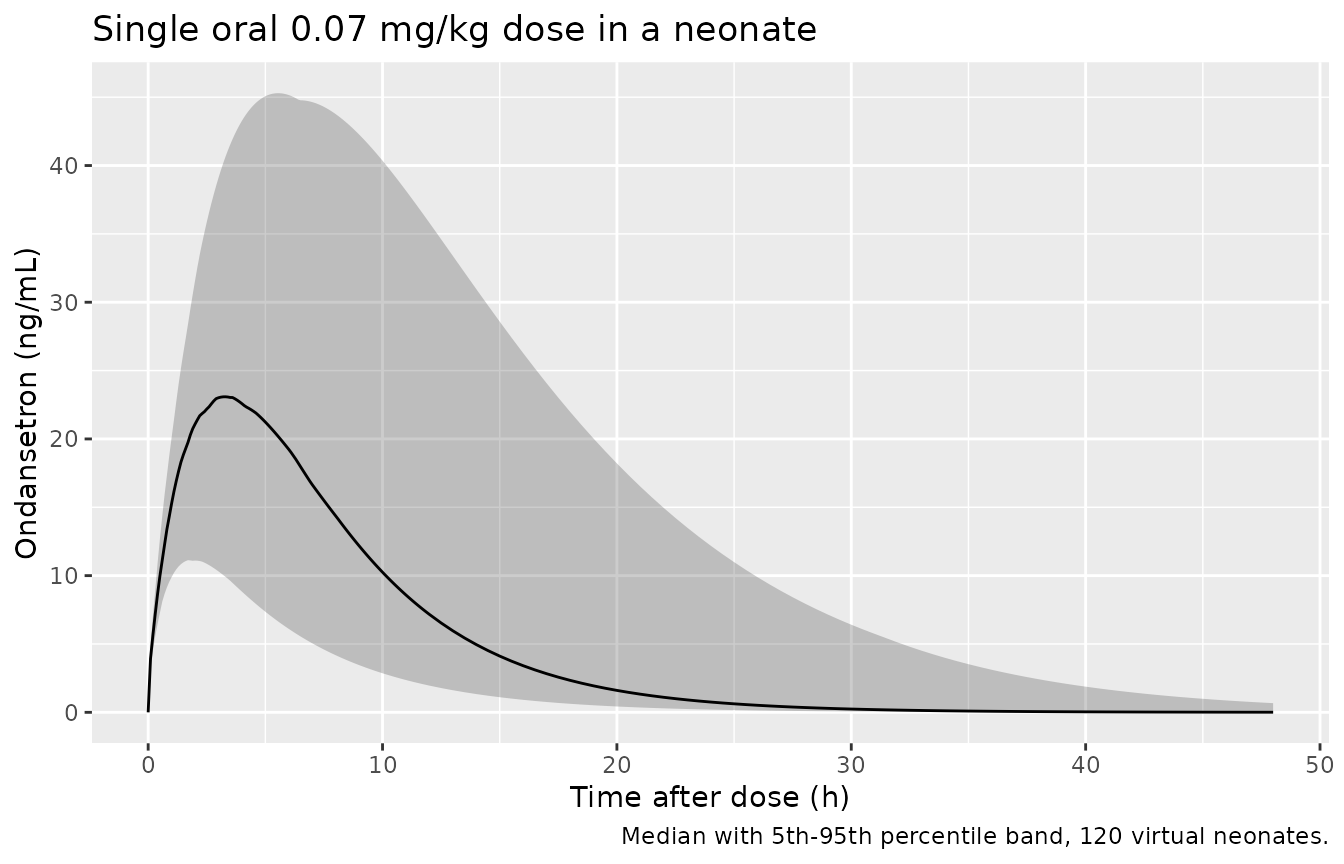
Absorption (KA = 0.19 /h) is far slower than disposition, so the profile is flip-flop: the terminal slope is set by KA rather than by elimination.
char_nca <- sim_char |>
  filter(!is.na(Cc)) |>
  select(id, time, Cc, arm)

char_nca <- bind_rows(
  char_nca,
  char_nca |> distinct(id, arm) |> mutate(time = 0, Cc = 0)
) |>
  distinct(id, arm, time, .keep_all = TRUE) |>
  arrange(id, arm, time)

char_dose <- char_events |>
  filter(evid == 1) |>
  select(id, time, amt, arm)

char_conc_obj <- PKNCA::PKNCAconc(char_nca, Cc ~ time | arm + id,
                                  concu = "ng/mL", timeu = "h")
char_dose_obj <- PKNCA::PKNCAdose(char_dose, amt ~ time | arm + id,
                                  doseu = "mg")

char_res <- PKNCA::pk.nca(PKNCA::PKNCAdata(
  char_conc_obj, char_dose_obj,
  intervals = data.frame(start = 0, end = Inf, cmax = TRUE, tmax = TRUE,
                         aucinf.obs = TRUE, half.life = TRUE)
))

char_tbl <- as.data.frame(char_res$result) |>
  # pk.nca() also returns the lambda-z regression diagnostics that back the
  # half-life; keep the four requested parameters.
  filter(PPTESTCD %in% c("cmax", "tmax", "aucinf.obs", "half.life")) |>
  group_by(PPTESTCD) |>
  summarise(Median = median(PPORRES, na.rm = TRUE),
            P05 = quantile(PPORRES, 0.05, na.rm = TRUE),
            P95 = quantile(PPORRES, 0.95, na.rm = TRUE), .groups = "drop") |>
  mutate(Parameter = nlmixr2lib::ncaParamLabel(PPTESTCD)) |>
  select(Parameter, Median, P05, P95)

knitr::kable(
  char_tbl, digits = 2,
  caption = "Non-compartmental characterisation of a single oral 0.07 mg/kg neonatal dose (120 virtual neonates)."
)| Parameter | Median | P05 | P95 |
|---|---|---|---|
| AUC0-∞ (obs) | 234.81 | 86.22 | 824.07 |
| Cmax | 23.12 | 11.18 | 45.32 |
| t½ | 3.69 | 3.66 | 5.49 |
| Tmax | 3.05 | 1.80 | 6.11 |
Structural identity: AUC0-inf equals F x Dose / CL
For a linear model with first-order input, the exact per-subject
identity AUC0-inf = F * Dose / CL holds regardless of the
absorption rate. Comparing the PKNCA result to the closed form is a
per-subject check on the whole pipeline (dosing units, the
f(depot) assignment, and the 1000 * unit
conversion in Cc), not a median-versus-median
comparison.
cl_i <- sim_char |> distinct(id, cl) |> arrange(id)

analytic_char <- char_subj |>
  left_join(cl_i, by = "id") |>
  mutate(auc_analytic = 1000 * f_bioav * dose_per_kg * WT_BIRTH / cl)

auc_check <- as.data.frame(char_res$result) |>
  filter(PPTESTCD == "aucinf.obs") |>
  select(id, auc_pknca = PPORRES) |>
  left_join(analytic_char |> select(id, auc_analytic), by = "id") |>
  mutate(rel_err = abs(auc_pknca - auc_analytic) / auc_analytic)

c(f = f_bioav,
  max_rel_err = max(auc_check$rel_err),
  median_rel_err = median(auc_check$rel_err))
#>              f    max_rel_err median_rel_err
#>   0.6200000000   0.0011110707   0.0003221375
stopifnot(max(auc_check$rel_err) < 0.02)
Trial replication: cumulative exposure by number of doses
Lam 2025 simulated, for each neonate, the cumulative AUC from birth
to tl (75 h after the last study dose) and the maximum
concentration over the same window, then plotted the change in mean
Finnegan scores against exposure quantiles stratified by the total
number of doses received (Figures 3 and 4). The PD layer is not a model
in the paper - the exposure-response analysis is graphical - so what is
reproduced here is the exposure (boxplot) layer of those figures.
trial_nca <- sim_trial |>
  filter(!is.na(Cc)) |>
  select(id, time, Cc, arm)

trial_nca <- bind_rows(
  trial_nca,
  trial_nca |> distinct(id, arm) |> mutate(time = 0, Cc = 0)
) |>
  distinct(id, arm, time, .keep_all = TRUE) |>
  arrange(id, arm, time)

trial_dose <- trial_events |>
  filter(evid == 1) |>
  select(id, time, amt, arm)

trial_conc_obj <- PKNCA::PKNCAconc(trial_nca, Cc ~ time | arm + id,
                                   concu = "ng/mL", timeu = "h")
trial_dose_obj <- PKNCA::PKNCAdose(trial_dose, amt ~ time | arm + id,
                                   doseu = "mg")

trial_res <- PKNCA::pk.nca(PKNCA::PKNCAdata(
  trial_conc_obj, trial_dose_obj,
  intervals = data.frame(start = 0, end = Inf, cmax = TRUE, tmax = TRUE,
                         auclast = TRUE)
))

exposure <- as.data.frame(trial_res$result) |>
  filter(PPTESTCD %in% c("cmax", "auclast")) |>
  select(arm, id, PPTESTCD, PPORRES) |>
  tidyr::pivot_wider(names_from = PPTESTCD, values_from = PPORRES) |>
  left_join(trial_events |> distinct(id, n_doses), by = "id")

# The paper's Cmax is the maximum from BIRTH to tl, so for a neonate whose
# maternal-transfer concentration exceeds every post-dose peak it is simply
# C0. Carry a post-first-dose maximum alongside it so the two contributions
# can be told apart in the comparison below.
cmax_postdose <- sim_trial |>
  filter(time >= first_dose_time) |>
  group_by(id) |>
  summarise(cmax_postdose = max(Cc), .groups = "drop")

exposure <- exposure |> left_join(cmax_postdose, by = "id")

# Every subject must have both metrics; an NA here would silently turn the
# arm-level medians and the attainment percentages below into NA.
stopifnot(
  nrow(exposure) == 4L * n_per_arm,
  !anyNA(exposure$auclast), !anyNA(exposure$cmax)
)
exposure |>
  tidyr::pivot_longer(c(auclast, cmax), names_to = "metric", values_to = "value") |>
  mutate(metric = factor(metric, levels = c("auclast", "cmax"),
                         labels = c("Cumulative AUC0-tl (ng*h/mL)",
                                    "Cmax (ng/mL)"))) |>
  ggplot(aes(x = factor(n_doses), y = value)) +
  geom_boxplot(outlier.size = 0.5) +
  facet_wrap(~metric, scales = "free_y") +
  scale_y_log10() +
  labs(x = "Total number of ondansetron doses received",
       y = NULL,
       title = "Exposure by number of doses",
       caption = paste("Replicates the exposure (boxplot) layer of Figures 3 and 4",
                       "of Lam 2025; the Finnegan-score layer is not a model."))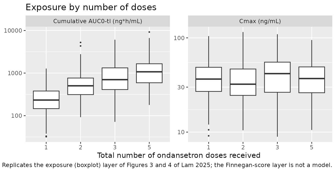
Comparison against published exposure landmarks
Lam 2025 publishes no NCA table. The quantitative exposure values it does report are the medians of the exposure quantiles shown in Figures 1-4, quoted in the Results text. The most completely specified stratum is the five-dose group, for which both metrics are given: a change in mean Finnegan scores of -3.59 units “between a median of 700 and 1650 ng*h/mL” (Figure 3) and “between a median of 19.6 and 37.5 ng/mL” for Cmax (Figure 4). The reference values below are the geometric midpoints of those reported quantile-median intervals, which is the closest single-number summary the paper supports; the interval itself is quoted alongside so a reader can see the width of the target.
published <- tibble::tribble(
  ~arm,      ~auclast, ~cmax,
  "5 doses", sqrt(700 * 1650), sqrt(19.6 * 37.5)
)

cmp <- nlmixr2lib::ncaComparisonTable(
  simulated = exposure |> filter(arm == "5 doses") |>
    tidyr::pivot_longer(c(auclast, cmax), names_to = "PPTESTCD",
                        values_to = "PPORRES") |>
    as.data.frame(),
  reference = published,
  by = "arm",
  units = c(auclast = "ng*h/mL", cmax = "ng/mL"),
  tolerance_pct = 20
)

knitr::kable(
  cmp, digits = 1,
  caption = paste(
    "Simulated (median of 120 virtual neonates) vs. the geometric midpoint of",
    "the quantile-median intervals reported by Lam 2025 for the five-dose",
    "stratum: AUC0-tl 700-1650 ng*h/mL (Figure 3), Cmax 19.6-37.5 ng/mL",
    "(Figure 4). * differs from reference by >20%."
  )
)| NCA parameter | arm | Reference | Simulated | % diff |
|---|---|---|---|---|
| Cmax (ng/mL) | 5 doses | 27.1 | 37 | +36.5%* |
| AUClast (ng*h/mL) | 5 doses | 1070 | 1070 | -0.2% |
The AUC row is the informative one. Cmax carries a known upward bias
in this reproduction: the paper defines Cmax as the maximum from
birth, so for a neonate whose maternal-transfer
concentration exceeds every post-dose peak it is simply C0,
and the virtual cohort assigns a maternal concentration drawn from
N(28.2, 23.5) ng/mL to every subject, whereas the trial
reports that only “more than half” of neonates had a measurable pre-dose
concentration. Separating the two contributions shows the size of that
effect:
exposure |>
  left_join(trial_events |> distinct(id, CP0_MAT_NGML), by = "id") |>
  group_by(arm) |>
  summarise(
    `Median maternal CP0_MAT_NGML (ng/mL)` = median(CP0_MAT_NGML),
    `Median Cmax from birth (ng/mL)` = median(cmax),
    `Median Cmax after the first dose (ng/mL)` = median(cmax_postdose),
    .groups = "drop"
  ) |>
  knitr::kable(digits = 1,
caption = "Cmax from birth (the paper's definition, which includes the maternal-transfer spike) vs. the post-dose maximum.")| arm | Median maternal CP0_MAT_NGML (ng/mL) | Median Cmax from birth (ng/mL) | Median Cmax after the first dose (ng/mL) |
|---|---|---|---|
| 1 dose | 34.0 | 36.5 | 22.9 |
| 2 doses | 25.3 | 32.2 | 25.4 |
| 3 doses | 33.1 | 41.7 | 24.3 |
| 5 doses | 31.8 | 37.0 | 22.8 |
exposure |>
  group_by(arm) |>
  summarise(
    `Median AUC0-tl (ng*h/mL)` = median(auclast),
    `Median Cmax (ng/mL)` = median(cmax),
    .groups = "drop"
  ) |>
  mutate(
    `Lam 2025 reported quantile-median interval` = c(
      "not reported", "not reported", "not reported",
      "AUC 700-1650 ng*h/mL; Cmax 19.6-37.5 ng/mL (Figures 3, 4)"
    )
  ) |>
  knitr::kable(
    digits = 1,
    caption = "Simulated median exposure by dose-count arm, with the published landmark where one exists."
)| arm | Median AUC0-tl (ng*h/mL) | Median Cmax (ng/mL) | Lam 2025 reported quantile-median interval |
|---|---|---|---|
| 1 dose | 232.8 | 36.5 | not reported |
| 2 doses | 502.9 | 32.2 | not reported |
| 3 doses | 701.4 | 41.7 | not reported |
| 5 doses | 1072.1 | 37.0 | AUC 700-1650 ng*h/mL; Cmax 19.6-37.5 ng/mL (Figures 3, 4) |
The whole-cohort landmarks reported elsewhere in the paper bracket the simulated values in the same way: Figure 2 quotes Cmax quantile medians of 19.6-37 ng/mL for the ondansetron-plus-morphine stratum, Figure S17 quotes 53.2-73.1 ng/mL for term neonates, and Figure 1 quotes cumulative AUC quantile medians of about 645 ngh/mL (ondansetron plus morphine) and about 1420 ngh/mL (ondansetron only).
Reproducing the “at least three doses” conclusion
The paper’s headline dosing conclusion is that “an AUC0-tl of at least 1000 ngh/mL appears to be the threshold for reducing mean Finnegan scores” and that “at least three doses of the current oral ondansetron regimen are required to reduce symptom severity”. Those two statements are jointly testable against the packaged model: with a typical CL the median neonate does not reach 1000 ngh/mL until four or five doses, but the large inter-individual variability in CL (84% CV) means a meaningful share of three-dose neonates does.
exposure |>
  group_by(arm) |>
  summarise(
    `Median AUC0-tl (ng*h/mL)` = median(auclast),
    `% reaching AUC0-tl >= 1000 ng*h/mL` = 100 * mean(auclast >= 1000),
    .groups = "drop"
  ) |>
  knitr::kable(digits = 1,
caption = "Attainment of the 1000 ng*h/mL cumulative-AUC landmark by number of doses.")| arm | Median AUC0-tl (ng*h/mL) | % reaching AUC0-tl >= 1000 ng*h/mL |
|---|---|---|
| 1 dose | 232.8 | 1.7 |
| 2 doses | 502.9 | 13.3 |
| 3 doses | 701.4 | 34.2 |
| 5 doses | 1072.1 | 52.5 |
attain <- exposure |>
  group_by(n_doses) |>
  summarise(pct = 100 * mean(auclast >= 1000), .groups = "drop") |>
  arrange(n_doses)
attain
#> # A tibble: 4 × 2
#>   n_doses   pct
#>     <int> <dbl>
#> 1       1  1.67
#> 2       2 13.3
#> 3       3 34.2
#> 4       5 52.5
# Attainment must increase monotonically with the number of doses, and the
# one-dose arm must be far below the three-dose arm.
stopifnot(
  all(diff(attain$pct) > 0),
  attain$pct[attain$n_doses == 1] < 10,
  attain$pct[attain$n_doses == 3] > 20
)
Structural identity for the cumulative AUC
The paper’s AUC0-tl is the integral of A_central / V
from birth to tl. Because tl sits many
terminal half-lives after the last dose, that integral is numerically
the total AUC, which for this linear model has the exact closed form
(A_maternal + n_doses * F * Dose) / CL. Checking PKNCA’s
trapezoidal AUC against the closed form per subject validates the
maternal initial condition and the multi-dose bookkeeping together.
cl_trial <- sim_trial |> distinct(id, cl)

auc_check_trial <- exposure |>
  left_join(trial_events |> distinct(id, WT_BIRTH, CP0_MAT_NGML), by = "id") |>
  left_join(cl_trial, by = "id") |>
  mutate(
    amt_total = CP0_MAT_NGML * vc_typ / 1000 +
      n_doses * f_bioav * dose_per_kg * WT_BIRTH,
    auc_analytic = 1000 * amt_total / cl,
    rel_err = abs(auclast - auc_analytic) / auc_analytic
  )

auc_check_trial |>
  group_by(arm) |>
  summarise(`Median relative error` = median(rel_err),
            `Max relative error` = max(rel_err), .groups = "drop") |>
  knitr::kable(digits = 4,
caption = "PKNCA trapezoidal AUC0-tl vs. the closed-form (A_maternal + n * F * Dose) / CL.")| arm | Median relative error | Max relative error |
|---|---|---|
| 1 dose | 0.0014 | 0.0077 |
| 2 doses | 0.0014 | 0.0211 |
| 3 doses | 0.0015 | 0.0071 |
| 5 doses | 0.0015 | 0.0070 |
Assumptions and deviations
-
Bioavailability is applied to the depot. Methods
2.2 states that “Bioavailability (F) was fixed to 0.62 for all model
runs” and Table 3 reports
F 0.62 (FIXED), so the packaged model appliesf(depot) <- 0.62. The Appendix S1 control stream agrees on the value but not on its use: it declares$THETA ... 0.49 FIX ;F, and 0.49 islogit(0.62) = log(0.62 / 0.38) = 0.4895(the five structural thetas in that block are log-transformed, as its; log transformed thetasheader says, butexp(0.49) = 1.63is not a possible bioavailability, so the F theta must be logit-scaled). What the printed stream lacks is anyF1 = ...assignment in$PKreferencing that theta, so as listed it declares a fixed F and never applies it - most likely an omission from the appendix listing. The paper’s prose and parameter table are taken as authoritative, and the published cumulative AUC independently discriminates the two readings. For a typical neonate (median CL 0.58 L/h, birth weight 3.19 kg) the closed-form cumulative AUC0-tl after five doses is1000 * (A_maternal + 5 * F * 0.07 * 3.19) / 0.58: with F = 0.62 that is about 1210 ngh/mL, which falls inside the 700-1650 ngh/mL quantile-median interval Lam 2025 reports for the five-dose stratum (Figure 3); with F = 1 it is about 1940 ngh/mL, roughly 18% above the top of that interval and 80% above its geometric midpoint. The simulated cohort above bears this out: the five-dose median cumulative AUC0-tl comes out within 0.2% of the 1070 ngh/mL geometric midpoint of the published interval, whereas F = 1 would scale it by(A_maternal + 5 * 0.07 * WT) / (A_maternal + 5 * 0.62 * 0.07 * WT), about 1.61x, to roughly 1720 ng*h/mL - above the top of the published interval and about 61% above its midpoint. Cmax does not discriminate (typical post-dose peak 24 ng/mL at F = 0.62 vs 39 ng/mL at F = 1, both inside the 19.6-73.1 ng/mL span of the published Cmax quantile medians), so the AUC comparison is what settles it. -
Additive residual SD taken as sqrt(80.9) = 8.99
ng/mL. Table 3 reports the sigma posterior median as 80.9 with
a parenthetical SD of 9.2, and the table note defines “SD of sigma =
sqrt(posterior median)”. Applying the paper’s own relationship to the
printed median gives 8.99, a 2% disagreement with the printed 9.2. The
value derived from the estimated quantity (the posterior median of the
variance) is used. The analogous IIV row is self-consistent to rounding:
the note’s formula
%CV = sqrt(exp(median) - 1) * 100applied to the printed 0.54 gives 84.6% against the printed 84.2%. -
No individual-level covariates. Allometric scaling
to 10.4 kg with fixed exponents (0.75 for CL and Q, 1 for V and V2) and
the clearance-maturation term
1 - beta_CL * exp(-(AGE - 1) * ln(2) / T_CL)with beta_CL = 0.76 and T_CL = 3.82 months are properties of the infant reference model. Lam 2025 used them once, at the cohort median birth weight and postmenstrual age, to compute the priors; the selected final model applies no covariate effect at the individual level (Results 3.1; Appendix S1$PK). The packaged model therefore has no covariates, and beta_CL / T_CL are documented rather than encoded asini()parameters, because encoding a parameter that the model body never uses would misrepresent the fit. - The infant reference model itself is not packaged. Lam 2025 cites it (reference 17) and reproduces its equations, but not its parameter values at the 10.4 kg reference weight, so it cannot be reconstructed from this paper alone.
-
Maternal transfer is encoded as a state initial condition,
driven by a covariate. The paper’s
A_0(2) = C0 * S2sets the neonatal central compartment toC0 * V / 1000mg at birth, and it lives in the$PKblock – it is part of the model, not a feature of the dataset. The packaged model reproduces it literally ascentral(0) <- CP0_MAT_NGML * vc / 1000, withCP0_MAT_NGML(the mother’s observed plasma concentration at delivery, ng/mL) declared incovariateDataand newly registered ininst/references/covariate-columns.md. Two consequences a downstream user should know. First,CP0_MAT_NGMLis a required covariate column: set it to 0 for a neonate with no transplacental transfer, as the characterisation arm above does. Second, because the initial condition is assigned insidemodel(), it takes precedence over anyinits =passed torxSolve(); that is the behaviour of the published model and matches how NONMEM’sA_0(2) =works. Delivering the same amount as a time-zeroevid = 1bolus intocentralwould be numerically equivalent, but it would push a structural feature of the paper’s model out of the model file and into every user’s event table. - Distributional assumptions for the virtual cohort. Birth weight is drawn as N(3.1, 0.4) kg truncated to 2.0-4.6 kg and the maternal plasma concentration as N(28.2, 23.5) ng/mL truncated to 0-120 ng/mL, matching the means and SDs in Table 1; the paper reports no distributional shape or per-subject values. In particular, every virtual neonate is given a maternal-transfer concentration, whereas the trial reports that only “more than half” of neonates had a measurable pre-dose concentration (29 maternal samples for 36 neonates); this biases the simulated Cmax from birth upward and is the reason that row is starred in the comparison table. The first neonatal dose is placed at 6 h, the midpoint of the protocol’s 4-8 h window.
- The exposure-response layer is not a model. Lam 2025’s Figures 1-4 plot average change in mean Finnegan scores against exposure quantiles; no PD model, hazard model or covariate-effect equation is estimated for that relationship, so nothing is packaged for it. Only the exposure (boxplot) layer of Figures 3 and 4 is reproduced here.
- Quantile-median references are not an NCA table. The reference values in the comparison table are geometric midpoints of the quantile-median intervals quoted in the Results text for the five-dose stratum, because the paper publishes no NCA summary. A direct quantile-by-quantile comparison would be misleading: the paper’s per-neonate exposures come from shrunk empirical-Bayes CL estimates on 1-5 samples per neonate, so their observed spread is much narrower than the estimated 84% CV population variability that the packaged model simulates.
Errata
No erratum or correction notice for Lam 2025 was found on the journal landing page, in PubMed, or in the PMC record (checked 2026-08-14). Two internal inconsistencies in the article itself are recorded above and handled explicitly: the Appendix S1 control stream never applies the bioavailability theta it declares, and Table 3’s parenthetical residual-error SD (9.2) does not equal the square root of the posterior median it is printed beside (sqrt(80.9) = 8.99).