Cholecalciferol (Lang 2023)
Source:vignettes/articles/Lang_2023_cholecalciferol.Rmd
Lang_2023_cholecalciferol.RmdModel and source
- Citation: Lang JE, Gonzalez Ramirez R, Balevic S, Bickel S, Hornik CP, Majure JM, Venkatachalam S, Snowden J, O’Sullivan B, James L. Pharmacokinetics of Oral Vitamin D in Children with Obesity and Asthma. Clin Pharmacokinet. 2023;62(11):1567. doi:10.1007/s40262-023-01285-9.
- Final model (VDORA Parts 1 and 2): Two-compartment population PK model of serum 25-hydroxyvitamin D (25(OH)D) after oral vitamin D3 (cholecalciferol) in children aged 6-17 years with asthma and overweight or obesity (VDORA Parts 1 and 2 combined, Lang 2023). First-order absorption of the vitamin D3 dose into the 25(OH)D central compartment, linear elimination, and a constant endogenous input that holds the pre-dose concentration at an estimated baseline (BASE). Clearance, central volume and intercompartmental clearance scale with the BMI-for-age z-score (fixed power exponents 0.75, 1 and 1; reference z-score 2.36). Doses are in nmol of vitamin D3 (1 IU = 0.025 ug = 0.0650 nmol) and concentrations in nmol/L of 25(OH)D (1 ng/mL = 2.496 nmol/L).
- Interim model (VDORA Part 1): Interim two-compartment population PK model of serum 25-hydroxyvitamin D (25(OH)D) after oral vitamin D3 (cholecalciferol) in children aged 6-17 years with asthma and overweight or obesity, fitted to VDORA Part 1 only (Lang 2023 Table 2) and used to choose the Part 2 dosing regimen. First-order absorption of the vitamin D3 dose into the 25(OH)D central compartment, linear elimination, and a constant endogenous input that holds the pre-dose concentration at an estimated baseline (BASE). No covariates. Doses are in nmol of vitamin D3 (1 IU = 0.025 ug = 0.0650 nmol) and concentrations in nmol/L of 25(OH)D (1 ng/mL = 2.496 nmol/L). The final model fitted to Parts 1 and 2 is Lang_2023_cholecalciferol.
- Article: https://doi.org/10.1007/s40262-023-01285-9 (open access; PMC10582143)
- Electronic Supplementary Material (ESM): covariate-model building tables (ESM Tables 1 and 3), prediction-error summary (ESM Table 2) and model diagnostics, available from the article page.
The VDORA study gave oral vitamin D3 (cholecalciferol) for 16 weeks to children with asthma and overweight or obesity and followed serum 25-hydroxyvitamin D (25(OH)D) for a further 12 weeks. The paper reports two population PK models, both packaged here:
-
Lang_2023_cholecalciferol_part1– the interim model fitted to the 44 children of Part 1 (Table 2). It has no covariates and was used to simulate candidate regimens (Table 3, Figures 2 and 3) and pick the Part 2 regimen (50,000 IU loading dose + 8000 IU daily). -
Lang_2023_cholecalciferol– the final model refitted to Parts 1 and 2 combined (Table 4, Eqs 7-9), with the BMI-for-age z-score scaling clearance, central volume and intercompartmental clearance.
Both models describe 25(OH)D, not vitamin D3 itself: the vitamin D3 dose is absorbed (first order, very slowly: Ka about 0.002 1/h, an absorption half-life near two weeks) directly into a two-compartment 25(OH)D disposition model, and a constant endogenous input keeps the untreated concentration at the estimated baseline BASE.
Units
The models work in molar units: doses in nmol of vitamin D3 and concentrations in nmol/L of 25(OH)D (BASE is reported in nmol/L). The paper reports doses in international units and its targets in ng/mL, so the vignette converts with
- 1 IU vitamin D3 = 0.025 ug; molecular weight 384.64 g/mol, so 1 IU = 0.0650 nmol (50,000 IU = 3250 nmol; 8000 IU = 520 nmol);
- 25(OH)D3 molecular weight 400.64 g/mol, so 1 ng/mL = 2.496 nmol/L (40 ng/mL = 99.8 nmol/L).
iu_to_nmol <- 0.025 * 1000 / 384.64 # nmol vitamin D3 per IU
nmolL_per_ngmL <- 1000 / 400.64 # nmol/L 25(OH)D per ng/mL
The paper does not state the dose unit used in the NONMEM data set. Dosing in nmol reproduces the published regimen simulations of Table 3 (below); dosing in ug would put the typical week-16 concentration on 50,000 IU + 8000 IU daily near 34 ng/mL, against the 82% of simulated children above 40 ng/mL that Table 3 reports, so the molar reading is the one consistent with the paper.
Population
The VDORA study (ClinicalTrials.gov NCT03686150) enrolled children aged 6-17 years with physician-diagnosed asthma, BMI at or above the 85th percentile for age and sex, and baseline serum 25(OH)D of 10 to < 30 ng/mL (Methods). Part 1 randomised 44 children (Table 1 cohorts A-D: 50,000 IU loading + 6000 IU daily, 50,000 IU loading + 10,000 IU daily, 6000 IU daily, 600 IU daily) and contributed 227 concentrations; Part 2 randomised 63 children 2:1 to 50,000 IU loading + 8000 IU daily (cohort E) or 600 IU daily (cohort F). The combined model used 848 concentrations from 109 children. Across the tabulated cohorts, median ages were 11.2-13.4 years, 48.6% were female, 41% White and 41% Black, 18% Hispanic, and 23 / 35 / 49 children were overweight / obese / morbidly obese (85th-95th / 95th-99th / >= 99th BMI percentile). Median baseline 25(OH)D was 14.5-21 ng/mL.
str(readModelDb("Lang_2023_cholecalciferol")()$population, give.attr = FALSE)
#> List of 12
#>  $ species       : chr "human"
#>  $ n_subjects    : num 109
#>  $ n_studies     : num 1
#>  $ age_range     : chr "6-17 years (Table 1 ranges 6.5-17.9 years)"
#>  $ age_median    : chr "11.2-13.4 years across the six dosing cohorts"
#>  $ weight_range  : chr "BMI at or above the 85th percentile for age and sex (BMI 17.5-53.1 kg/m^2)"
#>  $ sex_female_pct: num 48.6
#>  $ race_ethnicity: Named num [1:8] 41.1 41.1 3.7 0.9 1.9 4.7 6.5 17.8
#>  $ disease_state : chr "Physician-diagnosed asthma with overweight or obesity (BMI at or above the 85th percentile) and vitamin D insuf"| __truncated__
#>  $ dose_range    : chr "Oral vitamin D3 for 16 weeks: 50,000 IU loading dose + 6000, 8000 or 10,000 IU daily; 6000 IU daily without loa"| __truncated__
#>  $ regions       : chr "United States (multi-centre; ClinicalTrials.gov NCT03686150)"
#>  $ notes         : chr "VDORA study. 848 serum 25(OH)D concentrations from 109 children (46 Part 1, 63 Part 2) measured by immunoassay "| __truncated__
Source trace
| Equation / parameter | Final model (Parts 1+2) | Part 1 model | Source location |
|---|---|---|---|
| Two-compartment, first-order absorption, linear elimination | – | – | Results “Part 1 PK Model Development”; Methods “Combined Model Development” |
| Constant endogenous input; baseline BASE | kin = CL/F * BASE |
same | Results (“A constant endogenous input rate to the central compartment … A parameter (BASE) was used to describe the baseline”) |
lka (Ka, 1/h) |
0.0022 | 0.00178 | Table 4 / Table 2 |
lcl (CL/F, L/h) |
0.179 | 0.0858 | Table 4 / Table 2 |
lvc (Vc/F, L) |
30.2 | 35.2 | Table 4 / Table 2 |
lq (Q/F, L/h) |
0.116 | 0.189 | Table 4 / Table 2 |
lvp (Vp/F, L) |
170 | 724 | Table 4 / Table 2 |
lrbase (BASE, nmol/L) |
42.6 | 45.8 | Table 4 / Table 2 |
e_bmiz_cl (fixed) |
0.75 | – | Eq 7 |
e_bmiz_vc (fixed) |
1 | – | Eq 8 |
e_bmiz_q (fixed) |
1 | – | Eq 9 |
| BMIZ reference | 2.36 | – | Eqs 7-9 (cohort median z-score) |
etalcl (omega^2) |
0.63^2 | 1.13^2 | Table 4 / Table 2, IIV 63 / 113 %CV |
etalq (omega^2) |
1.20^2 | 0.28^2 | Table 4 / Table 2, IIV 120 / 28 %CV |
etalrbase (omega^2) |
0.30^2 | 0.27^2 | Table 4 / Table 2, IIV 30 / 27 %CV |
propSd |
0.15 | 0.13 | Table 4 / Table 2 |
Part 1 model: regimen simulations
Virtual cohort and simulation
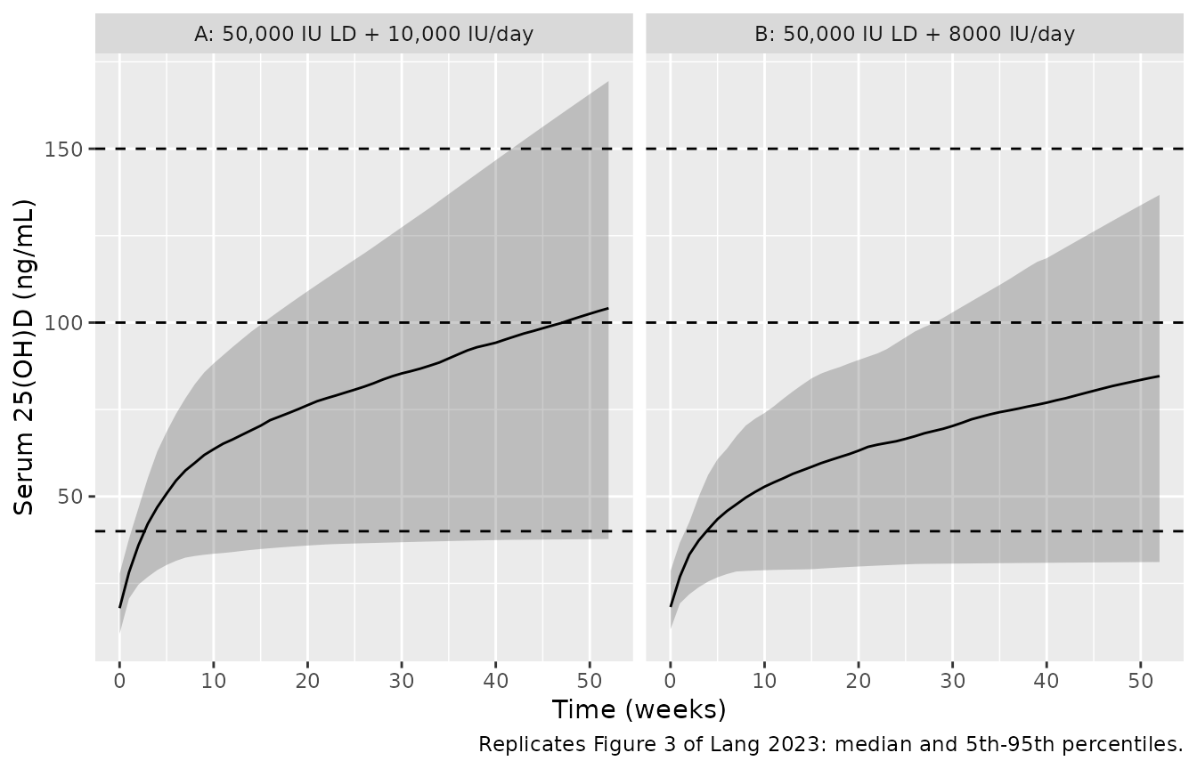
Part 1 simulated six regimens for 16 weeks in the 44 Part 1 children using their individual empirical Bayes estimates (Table 3, Figure 2), and two of them for 52 weeks (Figure 3). The individual estimates are not published, so the vignette draws 200 virtual children per regimen from the Part 1 model’s population distribution instead.
make_regimen <- function(n, ld_iu, md_iu, dose_weeks, obs_weeks, regimen,
                         id_offset = 0L, BMIZ = NULL) {
  ids <- id_offset + seq_len(n)
  daily <- tibble(
    id = ids, time = 0, amt = md_iu * iu_to_nmol, ii = 24,
    addl = dose_weeks * 7 - 1, evid = 1L, cmt = "depot"
  )
  loading <- if (ld_iu > 0) {
    tibble(id = ids, time = 0, amt = ld_iu * iu_to_nmol, ii = 0, addl = 0, evid = 1L, cmt = "depot")
  }
  obs <- tidyr::expand_grid(id = ids, time = obs_weeks * 7 * 24) |>
    mutate(amt = NA_real_, ii = 0, addl = 0, evid = 0L, cmt = "central")
  ev <- bind_rows(loading, daily, obs) |>
    mutate(regimen = regimen) |>
    arrange(id, time, desc(evid))
  if (!is.null(BMIZ)) {
    ev <- left_join(ev, tibble(id = ids, BMIZ = BMIZ), by = "id")
  }
  ev
}

regimens_p1 <- tibble::tribble(
  ~regimen, ~ld_iu, ~md_iu, ~pct40, ~pct100, ~pct150,
  "1: 50,000 IU LD + 10,000 IU/day", 50000, 10000, 98, 7, 0,
  "2: 50,000 IU LD + 9000 IU/day", 50000, 9000, 93, 2, 0,
  "3: 50,000 IU LD + 8000 IU/day", 50000, 8000, 82, 0, 0,
  "4: 50,000 IU LD + 5000 IU/day", 50000, 5000, 66, 0, 0,
  "5: 8000 IU/day", 0, 8000, 82, 0, 0,
  "6: 600 IU/day", 0, 600, 0, 0, 0
)

n_per_arm <- 200
events_p1 <- bind_rows(lapply(seq_len(nrow(regimens_p1)), function(i) {
  make_regimen(
    n_per_arm, regimens_p1$ld_iu[i], regimens_p1$md_iu[i],
    dose_weeks = 16, obs_weeks = 0:52, regimen = regimens_p1$regimen[i],
    id_offset = (i - 1L) * n_per_arm
  )
}))
stopifnot(!anyDuplicated(unique(events_p1[, c("id", "time", "evid", "amt")])))

mod_p1 <- readModelDb("Lang_2023_cholecalciferol_part1")
rxode2::rxSetSeed(2023)
sim_p1 <- rxode2::rxSolve(mod_p1, events = events_p1, keep = "regimen") |>
  as.data.frame() |>
  mutate(week = time / (7 * 24), conc_ngmL = Cc / nmolL_per_ngmL)
#> ℹ parameter labels from comments will be replaced by 'label()'
Table 3: target attainment at week 16
tab3 <- sim_p1 |>
  filter(week == 16) |>
  group_by(regimen) |>
  summarise(
    sim40 = 100 * mean(conc_ngmL >= 40),
    sim100 = 100 * mean(conc_ngmL >= 100),
    sim150 = 100 * mean(conc_ngmL >= 150),
    .groups = "drop"
  ) |>
  left_join(regimens_p1, by = "regimen")

tab3 |>
  select(regimen, pct40, sim40, pct100, sim100, pct150, sim150) |>
  rename(
    "Regimen" = regimen,
    ">= 40 ng/mL, published (%)" = pct40,
    ">= 40 ng/mL, simulated (%)" = sim40,
    ">= 100 ng/mL, published (%)" = pct100,
    ">= 100 ng/mL, simulated (%)" = sim100,
    ">= 150 ng/mL, published (%)" = pct150,
    ">= 150 ng/mL, simulated (%)" = sim150
  ) |>
knitr::kable(digits = 0, caption = "Replicates Table 3 of Lang 2023 (Part 1 model, 16 weeks of treatment).")| Regimen | >= 40 ng/mL, published (%) | >= 40 ng/mL, simulated (%) | >= 100 ng/mL, published (%) | >= 100 ng/mL, simulated (%) | >= 150 ng/mL, published (%) | >= 150 ng/mL, simulated (%) |
|---|---|---|---|---|---|---|
| 1: 50,000 IU LD + 10,000 IU/day | 98 | 92 | 7 | 10 | 0 | 0 |
| 2: 50,000 IU LD + 9000 IU/day | 93 | 88 | 2 | 4 | 0 | 0 |
| 3: 50,000 IU LD + 8000 IU/day | 82 | 88 | 0 | 1 | 0 | 0 |
| 4: 50,000 IU LD + 5000 IU/day | 66 | 71 | 0 | 0 | 0 | 0 |
| 5: 8000 IU/day | 82 | 88 | 0 | 0 | 0 | 0 |
| 6: 600 IU/day | 0 | 0 | 0 | 0 | 0 | 0 |
stopifnot(
  # The 40 ng/mL attainment depends on the dose (unit), CL/F and BASE together;
  # dosing in ug instead of nmol moves regimen 3 from about 82% to about 25%.
  # Observed while authoring: per-regimen differences of 0-6 points, which
  # are the gap between the population distribution sampled here and the
  # 44 shrunk individual estimates the paper simulated.
  median(abs(tab3$sim40 - tab3$pct40)) < 10,
  max(abs(tab3$sim40 - tab3$pct40)) < 20,
  # The paper's standard-of-care arm never reaches 40 ng/mL.
  tab3$sim40[tab3$md_iu == 600] < 5
)
The simulated attainment agrees with Table 3 to within a few percentage points for every regimen. The published percentages come from the 44 Part 1 children’s empirical Bayes estimates, whose spread is shrunk relative to the model’s population distribution, so the simulated tails (regimen 1’s attainment, the small fraction above 100 ng/mL) are slightly wider than published.
Figure 2: 16 weeks of treatment followed to week 52
sim_p1 |>
  group_by(regimen, week) |>
  summarise(
    q05 = quantile(conc_ngmL, 0.05), q50 = median(conc_ngmL),
    q95 = quantile(conc_ngmL, 0.95), .groups = "drop"
  ) |>
  ggplot(aes(week, q50)) +
  annotate("rect", xmin = 16, xmax = 52, ymin = -Inf, ymax = Inf, alpha = 0.1) +
  geom_ribbon(aes(ymin = q05, ymax = q95), alpha = 0.25) +
  geom_line() +
  geom_hline(yintercept = c(40, 100), linetype = "dashed") +
  facet_wrap(~regimen) +
  labs(
    x = "Time (weeks)", y = "Serum 25(OH)D (ng/mL)",
    caption = "Replicates Figure 2 of Lang 2023: median and 5th-95th percentiles; shaded = post-treatment."
  )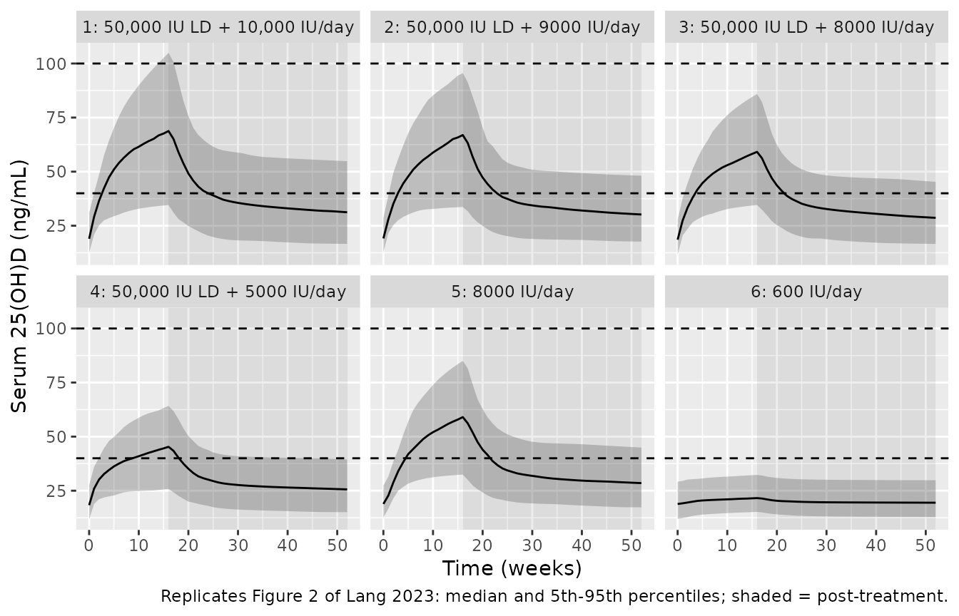
Figure 3: 52 weeks of treatment
events_52 <- bind_rows(
  make_regimen(n_per_arm, 50000, 10000, 52, 0:52, "A: 50,000 IU LD + 10,000 IU/day", 0L),
  make_regimen(n_per_arm, 50000, 8000, 52, 0:52, "B: 50,000 IU LD + 8000 IU/day", n_per_arm)
)
rxode2::rxSetSeed(2024)
sim_52 <- rxode2::rxSolve(mod_p1, events = events_52, keep = "regimen") |>
  as.data.frame() |>
  mutate(week = time / (7 * 24), conc_ngmL = Cc / nmolL_per_ngmL)

pub_52 <- tibble::tribble(
  ~regimen, ~pct40, ~pct100, ~pct150,
  "A: 50,000 IU LD + 10,000 IU/day", 98, 48, 7,
  "B: 50,000 IU LD + 8000 IU/day", 98, 27, 0
)
att_52 <- sim_52 |>
  filter(week == 52) |>
  group_by(regimen) |>
  summarise(
    sim40 = 100 * mean(conc_ngmL >= 40),
    sim100 = 100 * mean(conc_ngmL > 100),
    sim150 = 100 * mean(conc_ngmL > 150),
    .groups = "drop"
  ) |>
  left_join(pub_52, by = "regimen")

att_52 |>
  select(regimen, pct40, sim40, pct100, sim100, pct150, sim150) |>
  rename(
    "Regimen" = regimen,
    ">= 40 ng/mL, published (%)" = pct40,
    ">= 40 ng/mL, simulated (%)" = sim40,
    "> 100 ng/mL, published (%)" = pct100,
    "> 100 ng/mL, simulated (%)" = sim100,
    "> 150 ng/mL, published (%)" = pct150,
    "> 150 ng/mL, simulated (%)" = sim150
  ) |>
knitr::kable(digits = 0, caption = "Target attainment at week 52 (Results text accompanying Figure 3).")| Regimen | >= 40 ng/mL, published (%) | >= 40 ng/mL, simulated (%) | > 100 ng/mL, published (%) | > 100 ng/mL, simulated (%) | > 150 ng/mL, published (%) | > 150 ng/mL, simulated (%) |
|---|---|---|---|---|---|---|
| A: 50,000 IU LD + 10,000 IU/day | 98 | 92 | 48 | 54 | 7 | 14 |
| B: 50,000 IU LD + 8000 IU/day | 98 | 88 | 27 | 32 | 0 | 2 |
sim_52 |>
  group_by(regimen, week) |>
  summarise(
    q05 = quantile(conc_ngmL, 0.05), q50 = median(conc_ngmL),
    q95 = quantile(conc_ngmL, 0.95), .groups = "drop"
  ) |>
  ggplot(aes(week, q50)) +
  geom_ribbon(aes(ymin = q05, ymax = q95), alpha = 0.25) +
  geom_line() +
  geom_hline(yintercept = c(40, 100, 150), linetype = "dashed") +
  facet_wrap(~regimen) +
  labs(
    x = "Time (weeks)", y = "Serum 25(OH)D (ng/mL)",
    caption = "Replicates Figure 3 of Lang 2023: median and 5th-95th percentiles."
  )
Final model (Parts 1 and 2)
Virtual cohort
The BMI z-score distribution is not tabulated. The virtual cohort draws a z-score for each child from a normal distribution centred on the reported median of 2.36 (SD 0.6), truncated to 1.04-3.8: 1.04 is the z-score of the 85th percentile (the enrolment criterion) and 3.8 is a plausible upper end for severe paediatric obesity.
draw_bmiz <- function(n) {
  z <- numeric(0)
  while (length(z) < n) {
    x <- rnorm(n, 2.36, 0.6)
    z <- c(z, x[x >= 1.04 & x <= 3.8])
  }
  z[seq_len(n)]
}
set.seed(109)
events_p2 <- bind_rows(
  make_regimen(n_per_arm, 50000, 8000, 16, c(0, 1, 2, 4, 8, 12, 16, 20, 24, 28),
    "E: 50,000 IU LD + 8000 IU/day", 0L,
    BMIZ = draw_bmiz(n_per_arm)
  ),
  make_regimen(n_per_arm, 0, 600, 16, c(0, 1, 2, 4, 8, 12, 16, 20, 24, 28),
    "F: 600 IU/day", n_per_arm,
    BMIZ = draw_bmiz(n_per_arm)
  )
)
stopifnot(!anyDuplicated(unique(events_p2[, c("id", "time", "evid", "amt")])))

mod <- readModelDb("Lang_2023_cholecalciferol")
rxode2::rxSetSeed(2025)
sim_p2 <- rxode2::rxSolve(mod, events = events_p2, keep = c("regimen", "BMIZ")) |>
  as.data.frame() |>
  mutate(week = time / (7 * 24), conc_ngmL = Cc / nmolL_per_ngmL)
#> ℹ parameter labels from comments will be replaced by 'label()'
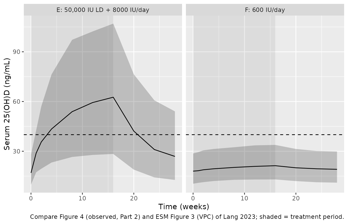
Figure 4 and ESM Figure 3: Part 2 concentration-time course
sim_p2 |>
  group_by(regimen, week) |>
  summarise(
    q05 = quantile(conc_ngmL, 0.05), q50 = median(conc_ngmL),
    q95 = quantile(conc_ngmL, 0.95), .groups = "drop"
  ) |>
  ggplot(aes(week, q50)) +
  annotate("rect", xmin = 0, xmax = 16, ymin = -Inf, ymax = Inf, alpha = 0.1) +
  geom_ribbon(aes(ymin = q05, ymax = q95), alpha = 0.25) +
  geom_line() +
  geom_hline(yintercept = 40, linetype = "dashed") +
  facet_wrap(~regimen) +
  labs(
    x = "Time (weeks)", y = "Serum 25(OH)D (ng/mL)",
    caption = "Compare Figure 4 (observed, Part 2) and ESM Figure 3 (VPC) of Lang 2023; shaded = treatment period."
  )
Part 2 target attainment at week 16
The Discussion reports that 79% of children on 50,000 IU + 8000 IU daily reached 40 ng/mL at week 16, none on 600 IU daily did, and 6% of those on the loading regimen exceeded 100 ng/mL.
att_p2 <- sim_p2 |>
  filter(week == 16) |>
  group_by(regimen) |>
  summarise(
    sim40 = 100 * mean(conc_ngmL >= 40),
    sim100 = 100 * mean(conc_ngmL > 100),
    median_ngmL = median(conc_ngmL),
    .groups = "drop"
  ) |>
  mutate(obs40 = c(79, 0), obs100 = c(6, 0))

att_p2 |>
  select(regimen, obs40, sim40, obs100, sim100, median_ngmL) |>
  rename(
    "Regimen" = regimen,
    ">= 40 ng/mL, observed (%)" = obs40,
    ">= 40 ng/mL, simulated (%)" = sim40,
    "> 100 ng/mL, observed (%)" = obs100,
    "> 100 ng/mL, simulated (%)" = sim100,
    "Simulated median (ng/mL)" = median_ngmL
  ) |>
knitr::kable(digits = 1, caption = "Week-16 attainment in Part 2: observed (Discussion) vs simulated (final model).")| Regimen | >= 40 ng/mL, observed (%) | >= 40 ng/mL, simulated (%) | > 100 ng/mL, observed (%) | > 100 ng/mL, simulated (%) | Simulated median (ng/mL) |
|---|---|---|---|---|---|
| E: 50,000 IU LD + 8000 IU/day | 79 | 86 | 6 | 11.5 | 62.6 |
| F: 600 IU/day | 0 | 1 | 0 | 0.0 | 21.3 |
The simulated attainment of 40 ng/mL on the loading regimen sits a few points above the observed 79%, and the simulated fraction above 100 ng/mL is somewhat above the observed 6%. The observed percentages come from the 43 children of cohort E, and the virtual cohort’s BMI z-score distribution is assumed (see Virtual cohort), so differences of this size are expected.
Table 5: concentrations by BMI z-score group
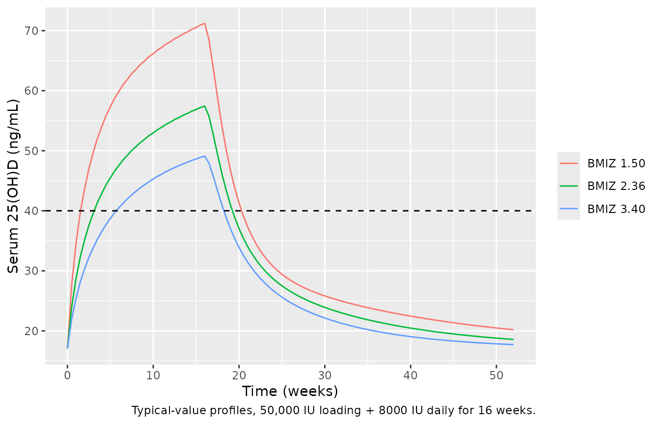
Table 5 tabulates week-16 predictions on 50,000 IU + 8000 IU daily by BMI z-score group. The typical-value curves below (no between-subject variability, BASE = 42.6 nmol/L) show the direction of the covariate effect: a higher z-score raises clearance and shortens the half-life, so both the rise during treatment and the post-treatment fall are faster.
typ_events <- bind_rows(lapply(seq_along(c(1.5, 2.36, 3.4)), function(i) {
  z <- c(1.5, 2.36, 3.4)[i]
  make_regimen(1, 50000, 8000, 16, seq(0, 52, by = 0.5),
    sprintf("BMIZ %.2f", z), i - 1L,
    BMIZ = z
  )
}))
# Three typical subjects that differ only in BMIZ; rxode2 warns that a
# multi-subject solve has no omega, which is the intent here.
sim_typ <- suppressWarnings(
  rxode2::rxSolve(rxode2::zeroRe(mod), events = typ_events, keep = c("regimen", "BMIZ"))
) |>
  as.data.frame() |>
  mutate(week = time / (7 * 24), conc_ngmL = Cc / nmolL_per_ngmL)
#> ℹ parameter labels from comments will be replaced by 'label()'
#> ℹ omega/sigma items treated as zero: 'etalcl', 'etalq', 'etalrbase'

ggplot(sim_typ, aes(week, conc_ngmL, colour = regimen)) +
  geom_line() +
  geom_hline(yintercept = 40, linetype = "dashed") +
  labs(
    x = "Time (weeks)", y = "Serum 25(OH)D (ng/mL)", colour = NULL,
    caption = "Typical-value profiles, 50,000 IU loading + 8000 IU daily for 16 weeks."
  )
sim_typ |>
  filter(week == 16) |>
  select(regimen, conc_ngmL) |>
  mutate(published_median_group = c(51, 49, 31)) |>
  rename(
    "BMI z-score" = regimen,
    "Typical week-16 concentration (ng/mL)" = conc_ngmL,
    "Table 5 population-predicted median of the group (ng/mL)" = published_median_group
  ) |>
knitr::kable(digits = 1)| BMI z-score | Typical week-16 concentration (ng/mL) | Table 5 population-predicted median of the group (ng/mL) |
|---|---|---|
| BMIZ 1.50 | 71.2 | 51 |
| BMIZ 2.36 | 57.4 | 49 |
| BMIZ 3.40 | 49.1 | 31 |
The typical-value concentrations fall with the z-score as in Table 5, but are higher than the Table 5 group medians (by about 20 ng/mL in the morbidly obese group). Table 5’s population predictions span 10-110 ng/mL within groups whose typical values differ by only a few ng/mL, so the tabulated predictions were not computed from the typical parameters alone; the table is reproduced here for orientation and not used as a gate.
PKNCA validation: 25(OH)D half-life by BMI z-score group
Table 5 reports the 25(OH)D elimination half-life by BMI z-score group (medians of the individual estimates). The half-life is computed here with PKNCA from the dose-attributable concentration (total 25(OH)D minus the individual baseline) after a single 50,000 IU dose, followed for up to three years so that the terminal phase is well sampled; dose-attributable concentrations below 0.01 nmol/L are dropped as below quantification. Time is converted to days so the half-life is in the paper’s unit.
nca_groups <- tibble::tribble(
  ~group, ~lo, ~hi,
  "Overweight (z 1.00-1.99)", 1.04, 1.99,
  "Obese (z 2.00-2.99)", 2.00, 2.99,
  "Morbidly obese (z >= 3.00)", 3.00, 3.80
)
set.seed(5)
events_nca <- bind_rows(lapply(seq_len(nrow(nca_groups)), function(i) {
  ids <- (i - 1L) * n_per_arm + seq_len(n_per_arm)
  z <- runif(n_per_arm, nca_groups$lo[i], nca_groups$hi[i])
  dose <- tibble(id = ids, time = 0, amt = 50000 * iu_to_nmol, evid = 1L, cmt = "depot")
  obs <- tidyr::expand_grid(id = ids, time = c(0, 1, 3, seq(7, 1092, by = 7)) * 24) |>
    mutate(amt = NA_real_, evid = 0L, cmt = "central")
  bind_rows(dose, obs) |>
    left_join(tibble(id = ids, BMIZ = z), by = "id") |>
    mutate(group = nca_groups$group[i]) |>
    arrange(id, time, desc(evid))
}))

rxode2::rxSetSeed(2026)
sim_nca <- rxode2::rxSolve(mod, events = events_nca, keep = c("group", "BMIZ")) |>
  as.data.frame() |>
  # Dose-attributable 25(OH)D. Below 0.01 nmol/L (1/4000 of the baseline) the
  # difference is ODE-solver noise around a ~40 nmol/L baseline, so those late
  # samples are treated as below quantification. At time 0 the difference
  # is zero up to floating-point rounding, so it is set to exactly 0.
  mutate(
    Cc = Cc - rbase,
    Cc = dplyr::case_when(time == 0 ~ 0, Cc < 0.01 ~ NA_real_, TRUE ~ Cc),
    time = time / 24
  ) |>
  filter(!is.na(Cc)) |>
  select(id, time, Cc, group)

conc_obj <- PKNCA::PKNCAconc(sim_nca, Cc ~ time | group + id)
dose_df <- events_nca |>
  filter(evid == 1) |>
  mutate(time = time / 24) |>
  select(id, time, amt, group)
dose_obj <- PKNCA::PKNCAdose(dose_df, amt ~ time | group + id)
intervals <- data.frame(
  start = 0, end = Inf, cmax = TRUE, tmax = TRUE, aucinf.obs = TRUE, half.life = TRUE
)
nca_res <- PKNCA::pk.nca(PKNCA::PKNCAdata(conc_obj, dose_obj, intervals = intervals))

published <- tibble::tribble(
  ~group, ~half.life,
  "Overweight (z 1.00-1.99)", 97.7,
  "Obese (z 2.00-2.99)", 65.9,
  "Morbidly obese (z >= 3.00)", 39.1
)
cmp <- nlmixr2lib::ncaComparisonTable(
  simulated = nca_res,
  reference = published,
  by = "group",
  units = c(cmax = "nmol/L", tmax = "day", aucinf.obs = "day*nmol/L", half.life = "day"),
  tolerance_pct = 20
)
knitr::kable(cmp, caption = "Simulated (single 50,000 IU dose) vs Table 5 median half-life. * differs from the reference by > 20%.")| NCA parameter | group | Reference | Simulated | % diff |
|---|---|---|---|---|
| t½ (day) | Overweight (z 1.00-1.99) | 97.7 | 103 | +4.9% |
| t½ (day) | Obese (z 2.00-2.99) | 65.9 | 77.8 | +18.0% |
| t½ (day) | Morbidly obese (z >= 3.00) | 39.1 | 59 | +50.9%* |
hl <- as.data.frame(nca_res$result) |>
  filter(PPTESTCD == "half.life") |>
  group_by(group) |>
  summarise(median_hl = median(PPORRES, na.rm = TRUE), .groups = "drop") |>
  left_join(published, by = "group")
stopifnot(
  # The BMI z-score effect (exponent 0.75 on CL/F, 1 on Vc/F and Q/F) must
  # shorten the half-life from the overweight to the morbidly obese group by
  # well over a third (published 97.7 -> 39.1 days).
  hl$median_hl[hl$group == "Morbidly obese (z >= 3.00)"] <
    0.75 * hl$median_hl[hl$group == "Overweight (z 1.00-1.99)"],
  # Magnitude: each group's median within a factor of 2 of Table 5 (observed
  # while authoring: ratios 1.1, 1.2 and 1.5, the last for the morbidly obese
  # group; see the narrative below).
  all(hl$median_hl / hl$half.life > 0.5 & hl$median_hl / hl$half.life < 2)
)
The simulated half-life falls steeply with the BMI z-score, reproducing the paper’s central covariate finding. The simulated group medians sit above the Table 5 medians, most in the morbidly obese group. Table 5’s half-lives are medians of the 109 children’s individual (empirical Bayes) estimates, which are shrunk towards the typical value and carry each child’s actual z-score, whereas the virtual cohort samples the full population distribution and spreads z-scores uniformly across each band; the paper itself notes that the fixed covariate exponents make the half-lives imprecise (Discussion).
Assumptions and deviations
- IIV of the final model. Table 4 tabulates the final-model IIV as 63% (CL/F), 120% (Q/F) and 30% (BASE), consistent with its own bootstrap column. The Results text describes these as the values before the BMI z-score was added and gives 59%, 104% and 29% after it; the Discussion quotes 61%, 96% and 29% for a body-weight model. Because the structural estimates of the final model are published only in Table 4, the maintainers used the Table 4 IIVs with them. Typical-value predictions are unaffected.
- IIV scale. The paper reports IIV as %CV for an exponential model. The printed RSEs of the IIV terms match the variance-scale RSE of CV = sqrt(omega^2) (for example, Part 1 CL/F: printed RSE 62%), so omega^2 = CV^2 rather than log(1 + CV^2).
- Dose unit. Doses are entered in nmol of vitamin D3 (see Units). The paper does not state the unit; the nmol reading is the one that reproduces Table 3.
- Endogenous input. The paper states that a constant endogenous input to the central compartment was used together with the baseline parameter BASE but does not print the equation. The model sets the input to CL/F x BASE and starts both disposition compartments at BASE, which keeps an undosed child at BASE and makes each dose add to it. Individual CL/F and BASE both carry IIV, so the input is individual.
- BMI z-score. The growth reference is not named. The covariate enters as a power of BMIZ / 2.36, so the model needs BMIZ > 0; it was developed in children at or above the 85th BMI percentile (z of about 1.04 or more) and should not be extrapolated to children of normal weight (Discussion).
- Virtual cohorts. The regimen simulations draw from the population distribution rather than the 44 Part 1 children’s individual estimates used by the paper, and the BMI z-score distribution of the final-model cohort is assumed (normal, mean 2.36, SD 0.6, truncated to 1.04-3.8).
- Loading dose timing. The loading dose is given together with the first daily dose at time 0.
- Not covered. Table 5’s predicted concentrations by z-score group are shown for orientation only (see above). No correction notice for the article was found as of 2026-11-07.