Sugemalimab population PK and exposure-survival in NSCLC (Sheng 2026)
Source:vignettes/articles/Sheng_2026_sugemalimab.Rmd
Sheng_2026_sugemalimab.RmdModel and source
Sheng 2026 used a population PK (popPK) model of sugemalimab, an anti-PD-L1 IgG4 antibody, to bridge the 1200 mg every-3-weeks (Q3W) dose studied in the all-Asian pivotal trial GEMSTONE-302 to heavier European patients with non-small-cell lung cancer (NSCLC). Exposure-response (ER) models for progression-free survival (PFS) and overall survival (OS), fitted to the GEMSTONE-302 sugemalimab arm, then translated the simulated exposures into survival probabilities. The paper reports four separately fitted models, packaged as four files:
modellib("Sheng_2026_sugemalimab")– two-compartment popPK model with time-decaying clearance.modellib("Sheng_2026_sugemalimab_pfs_inv")– PFS assessed by the investigator.modellib("Sheng_2026_sugemalimab_pfs_bicr")– PFS assessed by blinded independent central review (BICR).modellib("Sheng_2026_sugemalimab_os")– OS.Citation: Sheng Y, Yue Z, Xu F, Wang K, Wang J, Shi Q. Model-Informed Dosing Regimen of Sugemalimab for European Patients With Non-Small Cell Lung Cancer: Bridging From Asian Clinical Data. CPT Pharmacometrics Syst Pharmacol. 2026;15(3):e70220. doi:10.1002/psp4.70220. Parameter estimates from Supplementary Table S2; structure and covariate coding from the Supplementary Data S2 NONMEM control stream.
Article: https://doi.org/10.1002/psp4.70220
The popPK model is not the same fit as the sugemalimab model of Wang
2024 (modellib("Wang_2024_sugemalimab"), 1628 subjects from
nine trials, with a sigmoid time effect on clearance). Sheng 2026 uses a
separate analysis of 1002 subjects from six trials in which total
clearance is the sum of a time-independent and an exponentially decaying
component,
The three ER models are parametric time-to-event models driven by the
model-predicted trough concentration at the end of cycle 1
(CTROUGH, ug/mL; the paper’s
or CMINC1). Both PFS models use a Gompertz hazard with a
baseline that changes at 1 and 4 months; the OS model has a constant
hazard:
Time is in days in the PK model and in months in the ER models.
Population
The popPK model was fitted to 1002 adults from two Phase I, two Phase II and two Phase III studies (Sheng 2026 Table S1): median age 59 years (18-78), median weight 61 kg (36-124; 7.5% at or above 80 kg), median albumin 41.7 g/L, 22.6% female, 97.6% Asian. Tumour types were lymphoma (16.9%), stage III NSCLC (25.9%), stage IV NSCLC (35.3%) and other solid tumours (22.0%); 11.2% were ADA-positive. Almost all subjects (97.5%) received 1200 mg Q3W; the rest received 3-40 mg/kg.
The ER models were fitted to the 320 patients with stage IV NSCLC in the sugemalimab arm of GEMSTONE-302, who received 1200 mg Q3W with platinum-based chemotherapy. Their body weight ranged from 41 to 96 kg (mean 62 kg).
str(rxode2::rxode(readModelDb("Sheng_2026_sugemalimab"))$population)
#> ℹ parameter labels from comments will be replaced by 'label()'
#> List of 14
#>  $ species       : chr "human"
#>  $ n_subjects    : int 1002
#>  $ n_studies     : int 6
#>  $ age_range     : chr "18-78 years"
#>  $ age_median    : chr "59 years"
#>  $ weight_range  : chr "36-124 kg"
#>  $ weight_median : chr "61 kg"
#>  $ sex_female_pct: num 22.6
#>  $ race_ethnicity: Named num [1:3] 97.6 2 0.4
#>   ..- attr(*, "names")= chr [1:3] "Asian" "White" "Other"
#>  $ disease_state : chr "Adults with advanced solid tumours or lymphomas: lymphoma 169 (16.9%), stage III NSCLC 259 (25.9%), stage IV NS"| __truncated__
#>  $ dose_range    : chr "Sugemalimab IV 3, 10, 20 or 40 mg/kg (25 subjects) or 1200 mg (977 subjects, 97.5%) every 3 weeks."
#>  $ regions       : chr "Predominantly China (97.6% Asian)."
#>  $ ada_status    : chr "ADA-negative 890 (88.8%), ADA-positive 112 (11.2%)."
#>  $ notes         : chr "Baseline demographics from Sheng 2026 Table S1. Two Phase I, two Phase II and two Phase III studies (Table S1 s"| __truncated__
Source trace
Every ini() value carries an in-file comment naming its
source. Parameter estimates are from Supplementary Table S2 (popPK) and
Table S3 (ER); the model structure and the covariate coding are from the
NONMEM control streams in Supplementary Data S2.
| Parameter / equation | Value | Source |
|---|---|---|
lcl_exp_inf (CL0) |
log(0.149 L/day) | Table S2 |
lcl_exp_component (CLT at t = 0) |
log(0.108 L/day) | Table S2 |
lcl_exp_kdes (Kdes, non-lymphoma) |
log(0.0188 1/day) | Table S2 |
lcl_exp_kdes_lymph (Kdes, lymphoma) |
log(0.0465 1/day) | Table S2; control stream
IF(DSSTAT.EQ.1) TVKDES = THETA(13)
|
lvc, lq, lvp
|
log(3.42 L), log(0.373 L/day), log(0.573 L) | Table S2 |
e_wt_cl_exp_inf, e_alb_cl_exp_inf
|
0.770, -0.980 | Table S2; reference 61.5 kg and 41.9 g/L from the control stream and the main-text equations |
e_wt_vc, e_alb_vc,
e_alb_vp
|
0.446, -0.332, -1.40 | Table S2 |
e_sexf_cl_exp_inf,
e_sexf_cl_exp_component, e_sexf_vc
|
log(0.904), log(0.713), log(0.858) | Table S2; THETA**SEX in the control stream |
e_lymph_vc, e_nsclc_vp
|
log(0.896), log(3.21) | Table S2; DSVC, DSVP in the control
stream |
e_adatiter_cl_exp_component |
0.092 | Table S2;
TITERCOV = 1 + THETA(17)*(LOG(TITERLCF) - LOG(0.5))
|
| IIV CL0, Vc, CLT, Kdes, Vp | SD 0.249, 0.186, 0.463, 1.042, 0.616 | Table S2 (SD x 100, see Assumptions) |
| Correlations CL0-Vc, CLT-Vc, CLT-Kdes | 0.365, 0.610, 0.448 | Table S2; other correlations fixed to 0 in the control stream |
propSd |
0.169 | Table S2 |
CL = CLT * exp(-Kdes * t) + CL0, two-compartment
ODEs |
– | Control stream $DES; main-text equations |
PFS (investigator) lhaz_base_p1/p2/p3
|
log(0.039), log(0.099), log(0.282) per month | Table S3 |
PFS (investigator) gomp_haz,
e_ctrough_haz, e_pdl1neg_haz
|
-0.0638, log(0.908), log(1.457) | Table S3 |
PFS (BICR) lhaz_base_p1/p2/p3
|
log(0.043), log(0.16), log(0.347) per month | Table S3 |
PFS (BICR) gomp_haz, e_ctrough_haz,
e_pdl1neg_haz
|
-0.0768, log(0.876), log(1.485) | Table S3 |
OS lhaz_base, e_ctrough_haz
|
log(0.137) per month, log(0.798) | Table S3 |
| PFS hazard, baseline pieces at 1 and 4 months | – | Table S3 footnote; PFS control stream $DES
|
| OS constant hazard | – | Table S3 footnote; OS control stream $DES
|
Virtual cohorts
The individual data are not public. The simulations below use virtual cohorts built from the published summaries:
- Modelling cohort (Table S1): 22.55% female; lymphoma, NSCLC (stage III and IV) and other solid tumours in the proportions 169 : 613 : 220; albumin drawn from a normal distribution with the Table S1 mean and SD (41.6, 5.04 g/L) and held within the observed range.
- GEMSTONE-302-like cohort: all stage IV NSCLC; weight drawn from a normal distribution with mean 62 kg (Discussion) and the Table S1 SD of 11.7 kg, held within the observed 41-96 kg; sex and albumin as above.
All subjects are ADA-negative (ADA_TITER = 0.5), as in
the paper’s simulations. Infusions are assumed to last 1 hour (not
reported).
set.seed(20260226)
rxode2::rxSetSeed(20260226)

mod_pk <- rxode2::rxode(readModelDb("Sheng_2026_sugemalimab"))
#> ℹ parameter labels from comments will be replaced by 'label()'

clamp <- function(x, lo, hi) pmin(pmax(x, lo), hi)

draw_covariates <- function(n, wt, tumour = c("mix", "nsclc")) {
  tumour <- match.arg(tumour)
  grp <- if (tumour == "mix") {
    sample(c("LYMPH", "NSCLC", "OTHER"), n, replace = TRUE, prob = c(169, 613, 220))
  } else {
    rep("NSCLC", n)
  }
  data.frame(
    WT = wt,
    ALB = clamp(rnorm(n, 41.6, 5.04), 26.1, 60),
    SEXF = rbinom(n, 1, 0.2255),
    ADA_TITER = 0.5,
    TUMTP_LYMPH = as.integer(grp == "LYMPH"),
    TUMTP_NSCLC = as.integer(grp == "NSCLC")
  )
}

# One IV dose of `dose` mg as a 1-hour infusion at time 0 per subject, plus
# observation rows on the central compartment at `obs_times` (days).
make_events <- function(cov, dose, obs_times) {
  n <- nrow(cov)
  dosing <- data.frame(
    id = seq_len(n), time = 0, amt = dose, rate = dose * 24,
    evid = 1L, cmt = "central"
  )
  obs <- expand.grid(id = seq_len(n), time = obs_times)
  obs$amt <- 0
  obs$rate <- 0
  obs$evid <- 0L
  obs$cmt <- "central"
  bind_rows(dosing, obs) |>
    arrange(id, time, desc(evid)) |>
    left_join(cbind(id = seq_len(n), cov), by = "id")
}
Cycle-1 exposure in GEMSTONE-302-like patients (PKNCA)
A GEMSTONE-302-like cohort of 200 patients receives one 1200 mg dose; cycle-1 exposure is computed with PKNCA over the 21-day dosing interval. The paper does not print absolute exposure values. Its one absolute anchor is the clinical reference concentration: the 5th percentile of the observed in GEMSTONE-302 was 42.6 ug/mL.
n_gem <- 200
cov_gem <- draw_covariates(n_gem, clamp(rnorm(n_gem, 62, 11.7), 41, 96), "nsclc")
obs_c1 <- c(0, 1 / 24, 0.25, 0.5, 1, 2, 3, 5, 7, 10, 14, 17.5, 21)
ev_gem <- make_events(cov_gem, 1200, obs_c1)
sim_gem <- rxode2::rxSolve(mod_pk, ev_gem, returnType = "data.frame") |>
  mutate(treatment = "1200 mg Q3W")
conc_df <- sim_gem |>
  filter(!is.na(Cc)) |>
  select(id, time, Cc, treatment)
dose_df <- ev_gem |>
  filter(evid == 1) |>
  transmute(id, time, amt, duration = 1 / 24, treatment = "1200 mg Q3W")

o_conc <- PKNCAconc(conc_df, Cc ~ time | treatment + id)
o_dose <- PKNCAdose(dose_df, amt ~ time | treatment + id, route = "intravascular", duration = "duration")
intervals <- data.frame(start = 0, end = 21, cmax = TRUE, auclast = TRUE, ctrough = TRUE)
nca_res <- pk.nca(PKNCAdata(o_conc, o_dose, intervals = intervals))

nca_wide <- as.data.frame(nca_res) |>
  select(id, treatment, PPTESTCD, PPORRES) |>
  pivot_wider(names_from = PPTESTCD, values_from = PPORRES)

nca_wide |>
  summarise(
    across(c(cmax, auclast, ctrough), list(
      gmean = ~ exp(mean(log(.x))),
      p05 = ~ quantile(.x, 0.05),
      p95 = ~ quantile(.x, 0.95)
    ))
  ) |>
  pivot_longer(everything(), names_to = c("parameter", "stat"), names_sep = "_(?=[^_]+$)") |>
  pivot_wider(names_from = stat, values_from = value) |>
  mutate(parameter = recode(parameter,
    cmax = "Cmax,C1 (ug/mL)", auclast = "AUC0-21d,C1 (ug*day/mL)", ctrough = "Ctrough,C1 (ug/mL)"
  )) |>
  rename(
    "NCA parameter" = parameter, "Geometric mean" = gmean,
    "5th percentile" = p05, "95th percentile" = p95
  ) |>
knitr::kable(digits = 1, caption = "Simulated cycle-1 exposure, GEMSTONE-302-like cohort, 1200 mg Q3W.")| NCA parameter | Geometric mean | 5th percentile | 95th percentile |
|---|---|---|---|
| Cmax,C1 (ug/mL) | 368.3 | 260.6 | 511.9 |
| AUC0-21d,C1 (ug*day/mL) | 3156.4 | 2232.7 | 4520.9 |
| Ctrough,C1 (ug/mL) | 77.4 | 44.7 | 122.9 |
p05_ctrough <- unname(quantile(nca_wide$ctrough, 0.05))
pct_above_ref <- 100 * mean(nca_wide$ctrough >= 42.6)
c(sim_p05_ctrough = p05_ctrough, observed_p05_ctrough = 42.6, pct_at_or_above_42.6 = pct_above_ref)
#>      sim_p05_ctrough observed_p05_ctrough pct_at_or_above_42.6
#>              44.6721              42.6000              96.0000

# The 5th percentile of a simulated cohort is a tail statistic; it is compared
# with a wide band. A wrong clearance or volume moves it by far more than this.
stopifnot(p05_ctrough > 42.6 * 0.75, p05_ctrough < 42.6 * 1.33)
The simulated 5th percentile of lands close to the observed 42.6 ug/mL, so the model reproduces the absolute exposure of the pivotal population.
Weight strata and dose (Table 2, Figure 2)
The paper took the empirical-Bayes estimates of all 1002 modelled subjects, reassigned each a body weight drawn uniformly within a 5-kg stratum from 80 to 150 kg, and compared the geometric-mean cycle-1 exposure of each stratum and dose with the model-predicted exposure of GEMSTONE-302.
The paper’s GEMSTONE-302 reference exposures are not published, and its weight-stratum cohort is the whole modelling population (only 61% NSCLC; NSCLC has a three-fold larger peripheral volume and so a lower cycle-1 AUC). The absolute geometric-mean ratios therefore cannot be reproduced from the summary data. The shape of the weight effect can: dividing every ratio by the ratio of the 80-85 kg, 1200 mg stratum cancels the unknown reference, in the paper’s table and in the simulation alike.
The comparison uses typical values (no between-subject variability), averaged over the six sex-by-tumour-type classes of Table S1 on the log scale at each stratum’s mid-weight, the same quantity a geometric mean estimates.
mod_typ <- rxode2::zeroRe(mod_pk)
strata <- data.frame(lo = seq(80, 145, by = 5)) |>
  mutate(hi = lo + 5, wt_mid = lo + 2.5, stratum = paste0(lo, "-", hi))

classes <- expand.grid(SEXF = 0:1, grp = c("LYMPH", "NSCLC", "OTHER"), stringsAsFactors = FALSE) |>
  mutate(
    w = ifelse(SEXF == 1, 0.2255, 0.7745) * c(LYMPH = 169, NSCLC = 613, OTHER = 220)[grp] / 1002,
    TUMTP_LYMPH = as.integer(grp == "LYMPH"),
    TUMTP_NSCLC = as.integer(grp == "NSCLC")
  )

grid_typ <- tidyr::crossing(strata, classes, dose = c(1200, 1500, 1800)) |>
  mutate(id = row_number(), ALB = 41.6, ADA_TITER = 0.5, WT = wt_mid)

ev_typ <- make_events(
  grid_typ |> select(WT, ALB, SEXF, ADA_TITER, TUMTP_LYMPH, TUMTP_NSCLC),
  1200, obs_c1
) |>
  left_join(grid_typ |> select(id, dose), by = "id") |>
  mutate(amt = ifelse(evid == 1, dose, 0), rate = ifelse(evid == 1, dose * 24, 0))

# Typical-value solve over many subjects: rxode2 warns that no omega is used,
# which is the intent here, so only that warning is muffled.
sim_typ <- withCallingHandlers(
  suppressMessages(rxode2::rxSolve(mod_typ, ev_typ, returnType = "data.frame")),
  warning = function(w) {
    if (grepl("without 'omega'", conditionMessage(w), fixed = TRUE)) invokeRestart("muffleWarning")
  }
) |>
  left_join(grid_typ |> select(id, stratum, dose, w), by = "id")

exp_typ <- sim_typ |>
  group_by(id, stratum, dose, w) |>
  arrange(time, .by_group = TRUE) |>
  summarise(
    auc = sum(diff(time) * (head(Cc, -1) + tail(Cc, -1)) / 2),
    cmax = max(Cc),
    ctrough = Cc[time == 21],
    .groups = "drop"
  ) |>
  group_by(stratum, dose) |>
  summarise(across(c(auc, cmax, ctrough), ~ exp(sum(w * log(.x)) / sum(w))), .groups = "drop")
table2 <- tibble::tribble(
  ~stratum, ~dose, ~pct_ref, ~auc, ~ctrough, ~cmax,
  "80-85", 1200, 96.0, 1.022, 0.990, 0.960,
  "85-90", 1200, 95.6, 0.996, 0.958, 0.934,
  "90-95", 1200, 94.7, 0.974, 0.930, 0.912,
  "95-100", 1200, 93.3, 0.952, 0.902, 0.891,
  "100-105", 1200, 91.9, 0.932, 0.878, 0.871,
  "105-110", 1200, 90.4, 0.912, 0.854, 0.853,
  "110-115", 1200, 89.2, 0.894, 0.831, 0.836,
  "115-120", 1200, 86.8, 0.877, 0.810, 0.820,
  "120-125", 1200, 84.6, 0.861, 0.790, 0.805,
  "125-130", 1200, 82.4, 0.846, 0.771, 0.791,
  "130-135", 1200, 79.9, 0.831, 0.752, 0.777,
  "135-140", 1200, 77.4, 0.817, 0.735, 0.764,
  "140-145", 1200, 74.6, 0.803, 0.719, 0.752,
  "145-150", 1200, 72.0, 0.790, 0.703, 0.741,
  "80-85", 1500, 98.8, 1.277, 1.238, 1.199,
  "85-90", 1500, 98.4, 1.246, 1.199, 1.168,
  "90-95", 1500, 98.1, 1.217, 1.162, 1.139,
  "95-100", 1500, 98.1, 1.190, 1.129, 1.112,
  "100-105", 1500, 97.8, 1.165, 1.098, 1.088,
  "105-110", 1500, 97.6, 1.141, 1.068, 1.065,
  "110-115", 1500, 97.5, 1.118, 1.040, 1.044,
  "115-120", 1500, 96.7, 1.096, 1.012, 1.024,
  "120-125", 1500, 96.1, 1.076, 0.988, 1.005,
  "125-130", 1500, 95.4, 1.056, 0.964, 0.987,
  "130-135", 1500, 94.4, 1.038, 0.941, 0.971,
  "135-140", 1500, 93.5, 1.021, 0.919, 0.955,
  "140-145", 1500, 92.7, 1.004, 0.899, 0.940,
  "145-150", 1500, 91.3, 0.988, 0.879, 0.925,
  "80-85", 1800, 99.5, 1.532, 1.487, 1.438,
  "85-90", 1800, 99.2, 1.494, 1.439, 1.399,
  "90-95", 1800, 99.2, 1.461, 1.396, 1.366,
  "95-100", 1800, 99.1, 1.427, 1.355, 1.333,
  "100-105", 1800, 99.0, 1.397, 1.318, 1.304,
  "105-110", 1800, 98.8, 1.368, 1.282, 1.277,
  "110-115", 1800, 98.5, 1.341, 1.248, 1.252,
  "115-120", 1800, 98.5, 1.316, 1.216, 1.228,
  "120-125", 1800, 98.4, 1.291, 1.186, 1.205,
  "125-130", 1800, 98.4, 1.268, 1.157, 1.184,
  "130-135", 1800, 97.9, 1.246, 1.130, 1.164,
  "135-140", 1800, 97.7, 1.225, 1.104, 1.144,
  "140-145", 1800, 97.4, 1.205, 1.079, 1.127,
  "145-150", 1800, 97.3, 1.185, 1.056, 1.109
)

normalise <- function(d) {
  ref <- d |> filter(stratum == "80-85", dose == 1200)
  d |> mutate(auc = auc / ref$auc, ctrough = ctrough / ref$ctrough, cmax = cmax / ref$cmax)
}

trend <- normalise(exp_typ) |>
  pivot_longer(c(auc, ctrough, cmax), names_to = "metric", values_to = "simulated") |>
  inner_join(
    normalise(table2) |>
      pivot_longer(c(auc, ctrough, cmax), names_to = "metric", values_to = "published"),
    by = c("stratum", "dose", "metric")
  ) |>
  mutate(pct_diff = 100 * (simulated / published - 1))

trend |>
  filter(stratum %in% c("80-85", "115-120", "145-150")) |>
  mutate(metric = recode(metric, auc = "AUC,C1", ctrough = "Ctrough,C1", cmax = "Cmax,C1")) |>
  select(dose, stratum, metric, published, simulated, pct_diff) |>
  arrange(dose, metric, stratum) |>
  rename(
    "Dose (mg)" = dose, "Weight stratum (kg)" = stratum, "Metric" = metric,
    "Table 2, relative" = published, "Simulated, relative" = simulated, "% difference" = pct_diff
  ) |>
knitr::kable(digits = 3, caption = "Exposure relative to the 80-85 kg, 1200 mg stratum (Table 2 vs. simulation), selected strata.")| Dose (mg) | Weight stratum (kg) | Metric | Table 2, relative | Simulated, relative | % difference |
|---|---|---|---|---|---|
| 1200 | 115-120 | AUC,C1 | 0.858 | 0.856 | -0.297 |
| 1200 | 145-150 | AUC,C1 | 0.773 | 0.769 | -0.477 |
| 1200 | 80-85 | AUC,C1 | 1.000 | 1.000 | 0.000 |
| 1200 | 115-120 | Cmax,C1 | 0.854 | 0.854 | 0.017 |
| 1200 | 145-150 | Cmax,C1 | 0.772 | 0.772 | 0.018 |
| 1200 | 80-85 | Cmax,C1 | 1.000 | 1.000 | 0.000 |
| 1200 | 115-120 | Ctrough,C1 | 0.818 | 0.816 | -0.327 |
| 1200 | 145-150 | Ctrough,C1 | 0.710 | 0.706 | -0.525 |
| 1200 | 80-85 | Ctrough,C1 | 1.000 | 1.000 | 0.000 |
| 1500 | 115-120 | AUC,C1 | 1.072 | 1.069 | -0.274 |
| 1500 | 145-150 | AUC,C1 | 0.967 | 0.962 | -0.528 |
| 1500 | 80-85 | AUC,C1 | 1.250 | 1.250 | 0.039 |
| 1500 | 115-120 | Cmax,C1 | 1.067 | 1.068 | 0.114 |
| 1500 | 145-150 | Cmax,C1 | 0.964 | 0.965 | 0.154 |
| 1500 | 80-85 | Cmax,C1 | 1.249 | 1.250 | 0.083 |
| 1500 | 115-120 | Ctrough,C1 | 1.022 | 1.019 | -0.278 |
| 1500 | 145-150 | Ctrough,C1 | 0.888 | 0.883 | -0.553 |
| 1500 | 80-85 | Ctrough,C1 | 1.251 | 1.250 | -0.040 |
| 1800 | 115-120 | AUC,C1 | 1.288 | 1.283 | -0.335 |
| 1800 | 145-150 | AUC,C1 | 1.159 | 1.154 | -0.477 |
| 1800 | 80-85 | AUC,C1 | 1.499 | 1.500 | 0.065 |
| 1800 | 115-120 | Cmax,C1 | 1.279 | 1.281 | 0.180 |
| 1800 | 145-150 | Cmax,C1 | 1.155 | 1.158 | 0.244 |
| 1800 | 80-85 | Cmax,C1 | 1.498 | 1.500 | 0.139 |
| 1800 | 115-120 | Ctrough,C1 | 1.228 | 1.223 | -0.409 |
| 1800 | 145-150 | Ctrough,C1 | 1.067 | 1.060 | -0.666 |
| 1800 | 80-85 | Ctrough,C1 | 1.502 | 1.500 | -0.134 |
summary(trend$pct_diff)
#>     Min.  1st Qu.   Median     Mean  3rd Qu.     Max.
#> -0.66582 -0.38056 -0.14173 -0.15583  0.06521  0.28420

# Deterministic (typical-value) comparison, so the bound applies to every cell.
stopifnot(max(abs(trend$pct_diff)) < 3)
Across all 42 strata-by-dose cells and all three metrics, the weight and dose dependence of the packaged model matches Table 2 to within a few percent. The dose dependence is exactly linear, as in the paper (1500/1200 mg = 1.25 in every stratum).
The paper’s first column, the proportion of patients whose reaches 42.6 ug/mL, depends on between-subject variability, so it is simulated stochastically: 200 subjects per stratum from the modelling cohort, with weight uniform within the stratum. The paper’s own cohort used the empirical-Bayes estimates of the 1002 modelled subjects, so this is an approximate reproduction.
cov_str <- strata |>
  rowwise() |>
  mutate(cov = list(draw_covariates(200, runif(200, lo, hi), "mix"))) |>
  ungroup() |>
  tidyr::unnest(cov) |>
  mutate(id = row_number())
ev_str <- make_events(
  cov_str |> select(WT, ALB, SEXF, ADA_TITER, TUMTP_LYMPH, TUMTP_NSCLC),
  1200, 21
)
sim_str <- rxode2::rxSolve(mod_pk, ev_str, returnType = "data.frame") |>
  filter(time == 21) |>
  left_join(cov_str |> select(id, stratum), by = "id")

# Linear PK: the 1500 and 1800 mg troughs are 1.25 and 1.5 times the 1200 mg
# trough of the same subject.
pct_ref <- tidyr::crossing(sim_str |> select(id, stratum, Cc), dose = c(1200, 1500, 1800)) |>
  group_by(stratum, dose) |>
  summarise(simulated = 100 * mean(Cc * dose / 1200 >= 42.6), .groups = "drop") |>
  inner_join(table2 |> select(stratum, dose, published = pct_ref), by = c("stratum", "dose")) |>
  mutate(diff_points = simulated - published)

pct_ref |>
  filter(stratum %in% c("80-85", "110-115", "115-120", "145-150")) |>
  rename(
    "Weight stratum (kg)" = stratum, "Dose (mg)" = dose,
    "Table 2: % >= 42.6 ug/mL" = published, "Simulated: % >= 42.6 ug/mL" = simulated,
    "Difference (points)" = diff_points
  ) |>
knitr::kable(digits = 1, caption = "Percentage of patients with Ctrough,C1 >= 42.6 ug/mL (Table 2 column 1), selected strata.")| Weight stratum (kg) | Dose (mg) | Simulated: % >= 42.6 ug/mL | Table 2: % >= 42.6 ug/mL | Difference (points) |
|---|---|---|---|---|
| 110-115 | 1200 | 86.0 | 89.2 | -3.2 |
| 110-115 | 1500 | 96.0 | 97.5 | -1.5 |
| 110-115 | 1800 | 98.5 | 98.5 | 0.0 |
| 115-120 | 1200 | 74.5 | 86.8 | -12.3 |
| 115-120 | 1500 | 92.0 | 96.7 | -4.7 |
| 115-120 | 1800 | 99.0 | 98.5 | 0.5 |
| 145-150 | 1200 | 67.0 | 72.0 | -5.0 |
| 145-150 | 1500 | 87.0 | 91.3 | -4.3 |
| 145-150 | 1800 | 93.0 | 97.3 | -4.3 |
| 80-85 | 1200 | 92.5 | 96.0 | -3.5 |
| 80-85 | 1500 | 99.0 | 98.8 | 0.2 |
| 80-85 | 1800 | 99.5 | 99.5 | 0.0 |
ggplot(
  tidyr::crossing(sim_str |> select(stratum, Cc), dose = c(1200, 1500, 1800)) |>
    mutate(Ctrough = Cc * dose / 1200, stratum = factor(stratum, levels = strata$stratum)),
  aes(stratum, Ctrough)
) +
  geom_boxplot(outlier.size = 0.4) +
  geom_hline(yintercept = 42.6, linetype = "dashed") +
  facet_wrap(~ paste(dose, "mg Q3W"), ncol = 1) +
  labs(x = "Body-weight stratum (kg)", y = "Ctrough,C1 (ug/mL)") +
  theme_bw() +
  theme(axis.text.x = element_text(angle = 45, hjust = 1))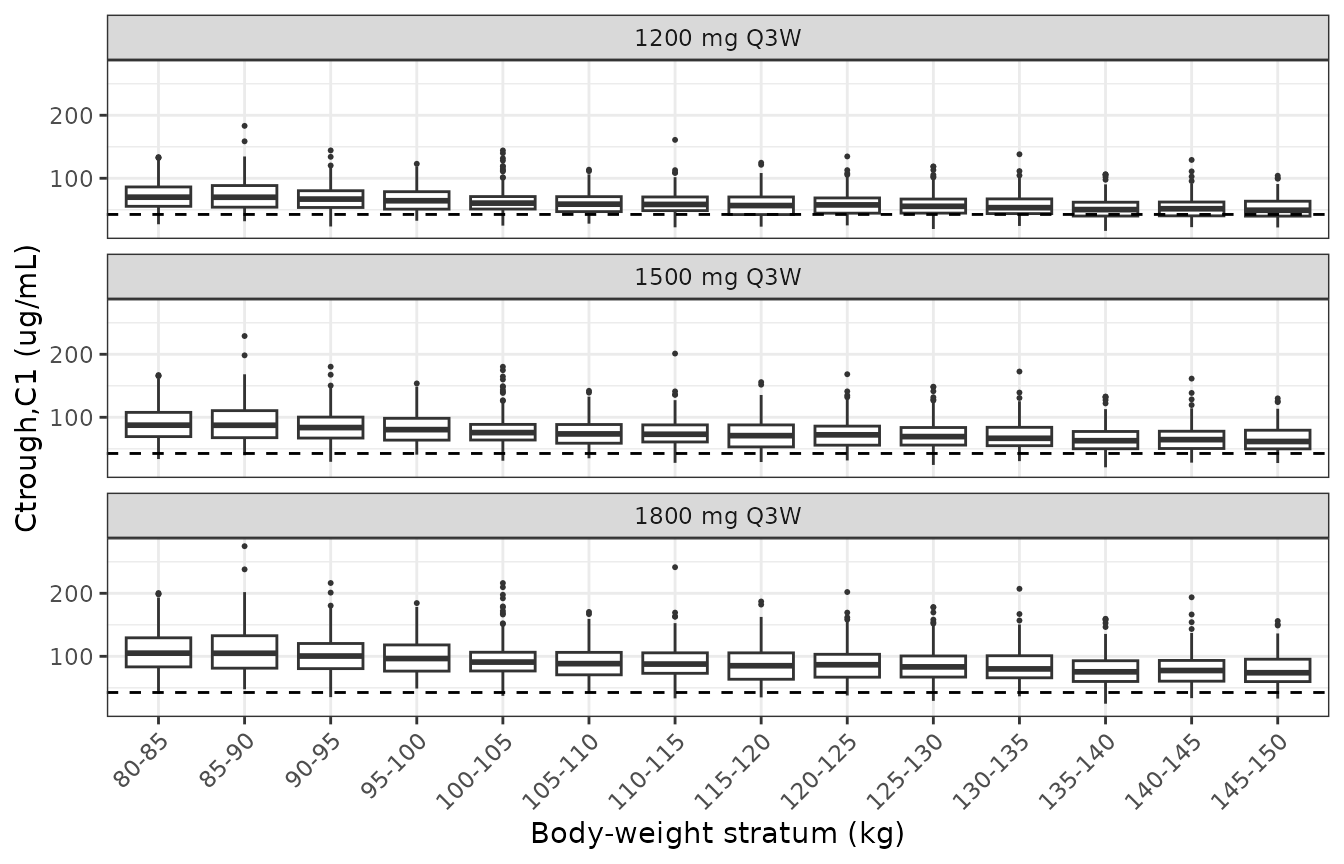
Replicates the Ctrough panel of Figure 2 of Sheng 2026 (dashed line: the 42.6 ug/mL clinical reference concentration).
Survival under the proposed regimen (Table 3, Figure 3)
The paper simulated three groups: Asian patients at 1200 mg (mimicking GEMSTONE-302), patients of 80-115 kg at 1200 mg, and patients of 115-150 kg at the proposed 1500 mg. Each virtual patient’s from the popPK model drives the three ER models. Here each group has 200 GEMSTONE-302-like patients (stage IV NSCLC); weight follows the GEMSTONE-302-like distribution for the Asian group and is uniform within the range for the other two.
groups <- tibble::tibble(
  group = c("Asian (1200 mg Q3W)", "80-115 kg (1200 mg Q3W)", "115-150 kg (1500 mg Q3W)"),
  dose = c(1200, 1200, 1500)
)
n_er <- 200
cov_er <- bind_rows(
  draw_covariates(n_er, clamp(rnorm(n_er, 62, 11.7), 41, 96), "nsclc"),
  draw_covariates(n_er, runif(n_er, 80, 115), "nsclc"),
  draw_covariates(n_er, runif(n_er, 115, 150), "nsclc")
) |>
  mutate(id = row_number(), group = rep(groups$group, each = n_er), dose = rep(groups$dose, each = n_er))

ev_er <- make_events(cov_er |> select(WT, ALB, SEXF, ADA_TITER, TUMTP_LYMPH, TUMTP_NSCLC), 1200, 21) |>
  left_join(cov_er |> select(id, dose), by = "id") |>
  mutate(amt = ifelse(evid == 1, dose, 0), rate = ifelse(evid == 1, dose * 24, 0))

ctrough_er <- rxode2::rxSolve(mod_pk, ev_er, returnType = "data.frame") |>
  filter(time == 21) |>
  select(id, CTROUGH = Cc) |>
  left_join(cov_er |> select(id, group), by = "id")

ctrough_er |>
  group_by(group) |>
  summarise(median = median(CTROUGH), p05 = quantile(CTROUGH, 0.05), p95 = quantile(CTROUGH, 0.95)) |>
  rename("Group" = group, "Median Ctrough,C1" = median, "5th pct" = p05, "95th pct" = p95) |>
knitr::kable(digits = 1, caption = "Simulated Ctrough,C1 (ug/mL) by group (compare Figure S6).")| Group | Median Ctrough,C1 | 5th pct | 95th pct |
|---|---|---|---|
| 115-150 kg (1500 mg Q3W) | 66.0 | 37.4 | 105.9 |
| 80-115 kg (1200 mg Q3W) | 60.8 | 37.1 | 96.8 |
| Asian (1200 mg Q3W) | 77.0 | 45.6 | 123.0 |
The ER models carry no random effects, so each patient’s survival curve follows from their and, for PFS, PD-L1 status. The paper sampled PD-L1 status from GEMSTONE-302 but does not report its distribution, so the curves are computed for both PD-L1 strata.
er_models <- c(
  "PFS (investigator)" = "Sheng_2026_sugemalimab_pfs_inv",
  "PFS (BICR)" = "Sheng_2026_sugemalimab_pfs_bicr",
  "OS" = "Sheng_2026_sugemalimab_os"
)
months <- seq(0, 24, by = 0.25)

er_input <- tidyr::crossing(ctrough_er, PDL1_TUM_POS = c(1L, 0L)) |>
  mutate(sid = row_number())

surv <- bind_rows(lapply(names(er_models), function(endpoint) {
  mod_er <- rxode2::rxode(readModelDb(er_models[[endpoint]]))
  ev <- tidyr::crossing(id = er_input$sid, time = months) |>
    mutate(evid = 0L, cmt = "cumhaz") |>
    left_join(er_input |> select(id = sid, CTROUGH, PDL1_TUM_POS), by = "id")
  rxode2::rxSolve(mod_er, ev, returnType = "data.frame") |>
    select(id, time, sur) |>
    left_join(er_input |> select(id = sid, group, PDL1_TUM_POS), by = "id") |>
    mutate(endpoint = endpoint)
}))
table3 <- tibble::tribble(
  ~endpoint, ~group, ~time, ~published,
  "PFS (investigator)", "Asian (1200 mg Q3W)", 12, 0.386,
  "PFS (investigator)", "80-115 kg (1200 mg Q3W)", 12, 0.344,
  "PFS (investigator)", "115-150 kg (1500 mg Q3W)", 12, 0.353,
  "PFS (investigator)", "Asian (1200 mg Q3W)", 24, 0.205,
  "PFS (investigator)", "80-115 kg (1200 mg Q3W)", 24, 0.170,
  "PFS (investigator)", "115-150 kg (1500 mg Q3W)", 24, 0.178,
  "PFS (BICR)", "Asian (1200 mg Q3W)", 12, 0.411,
  "PFS (BICR)", "80-115 kg (1200 mg Q3W)", 12, 0.353,
  "PFS (BICR)", "115-150 kg (1500 mg Q3W)", 12, 0.366,
  "PFS (BICR)", "Asian (1200 mg Q3W)", 24, 0.251,
  "PFS (BICR)", "80-115 kg (1200 mg Q3W)", 24, 0.199,
  "PFS (BICR)", "115-150 kg (1500 mg Q3W)", 24, 0.210,
  "OS", "Asian (1200 mg Q3W)", 12, 0.722,
  "OS", "80-115 kg (1200 mg Q3W)", 12, 0.636,
  "OS", "115-150 kg (1500 mg Q3W)", 12, 0.657,
  "OS", "Asian (1200 mg Q3W)", 24, 0.522,
  "OS", "80-115 kg (1200 mg Q3W)", 24, 0.405,
  "OS", "115-150 kg (1500 mg Q3W)", 24, 0.432
)

sim_t3 <- surv |>
  filter(time %in% c(12, 24)) |>
  group_by(endpoint, group, time, PDL1_TUM_POS) |>
  summarise(median_sur = median(sur), .groups = "drop") |>
  pivot_wider(names_from = PDL1_TUM_POS, values_from = median_sur, names_prefix = "pdl1_")

t3_cmp <- table3 |>
  left_join(sim_t3, by = c("endpoint", "group", "time")) |>
  mutate(
    lower = pmin(pdl1_0, pdl1_1), upper = pmax(pdl1_0, pdl1_1),
    bracketed = published >= lower & published <= upper,
    os_pct_diff = 100 * (pdl1_1 / published - 1)
  )

t3_cmp |>
  select(endpoint, group, time, published, pdl1_1, pdl1_0) |>
  rename(
    "Endpoint" = endpoint, "Group" = group, "Month" = time,
    "Table 3 median" = published,
    "Simulated median, PD-L1 >= 1% or missing" = pdl1_1,
    "Simulated median, PD-L1 < 1%" = pdl1_0
  ) |>
knitr::kable(digits = 3, caption = "Median survival probability at 12 and 24 months: Table 3 of Sheng 2026 vs. simulation by PD-L1 stratum.")| Endpoint | Group | Month | Table 3 median | Simulated median, PD-L1 >= 1% or missing | Simulated median, PD-L1 < 1% |
|---|---|---|---|---|---|
| PFS (investigator) | Asian (1200 mg Q3W) | 12 | 0.386 | 0.454 | 0.316 |
| PFS (investigator) | 80-115 kg (1200 mg Q3W) | 12 | 0.344 | 0.397 | 0.260 |
| PFS (investigator) | 115-150 kg (1500 mg Q3W) | 12 | 0.353 | 0.415 | 0.278 |
| PFS (investigator) | Asian (1200 mg Q3W) | 24 | 0.205 | 0.269 | 0.148 |
| PFS (investigator) | 80-115 kg (1200 mg Q3W) | 24 | 0.170 | 0.215 | 0.107 |
| PFS (investigator) | 115-150 kg (1500 mg Q3W) | 24 | 0.178 | 0.232 | 0.119 |
| PFS (BICR) | Asian (1200 mg Q3W) | 12 | 0.411 | 0.492 | 0.349 |
| PFS (BICR) | 80-115 kg (1200 mg Q3W) | 12 | 0.353 | 0.416 | 0.271 |
| PFS (BICR) | 115-150 kg (1500 mg Q3W) | 12 | 0.366 | 0.440 | 0.296 |
| PFS (BICR) | Asian (1200 mg Q3W) | 24 | 0.251 | 0.333 | 0.195 |
| PFS (BICR) | 80-115 kg (1200 mg Q3W) | 24 | 0.199 | 0.256 | 0.132 |
| PFS (BICR) | 115-150 kg (1500 mg Q3W) | 24 | 0.210 | 0.280 | 0.151 |
| OS | Asian (1200 mg Q3W) | 12 | 0.722 | 0.749 | 0.749 |
| OS | 80-115 kg (1200 mg Q3W) | 12 | 0.636 | 0.659 | 0.659 |
| OS | 115-150 kg (1500 mg Q3W) | 12 | 0.657 | 0.690 | 0.690 |
| OS | Asian (1200 mg Q3W) | 24 | 0.522 | 0.560 | 0.560 |
| OS | 80-115 kg (1200 mg Q3W) | 24 | 0.405 | 0.434 | 0.434 |
| OS | 115-150 kg (1500 mg Q3W) | 24 | 0.432 | 0.476 | 0.476 |
pfs_cmp <- filter(t3_cmp, endpoint != "OS")
os_cmp <- filter(t3_cmp, endpoint == "OS")
os_cmp$os_pct_diff
#> [1]  3.685784  3.622045  5.025285  7.359955  7.241749 10.213729

stopifnot(
  # PFS: the published value mixes the two PD-L1 strata in an unreported
  # proportion, so it must lie between the strata medians. The two strata are
  # separated by a hazard ratio of about 1.46, far wider than cohort noise.
  all(pfs_cmp$bracketed),
  # OS has no PD-L1 term. Centre and envelope, not every cell (see text).
  abs(median(os_cmp$os_pct_diff)) < 10,
  max(abs(os_cmp$os_pct_diff)) < 20
)
For PFS the published medians, which pool PD-L1 strata in the GEMSTONE-302 proportions, fall between the two simulated strata. For OS, which has no PD-L1 term, the simulated medians run about 4-10% above Table 3, more at 24 months than at 12. The direction is the one expected from the exposure checks above: the virtual GEMSTONE-302-like cohort’s 5th-percentile trough is a few percent above the observed 42.6 ug/mL, so its troughs, and with them its survival, run slightly high. The OS hazard ratio of 0.798 per 10 ug/mL turns a 10% higher trough (about 7 ug/mL) into a 15% lower hazard. The pivotal cohort’s albumin and sex distributions, which would explain the difference, are not reported. The group ordering matches the paper: the Asian group has the best survival, and raising the dose to 1500 mg for patients over 115 kg brings them above the 80-115 kg group at 1200 mg.
surv |>
  filter(PDL1_TUM_POS == 1L) |>
  group_by(endpoint, group, time) |>
  summarise(
    median = median(sur), lo = quantile(sur, 0.05), hi = quantile(sur, 0.95),
    .groups = "drop"
  ) |>
  ggplot(aes(time, median, colour = group, fill = group)) +
  geom_ribbon(aes(ymin = lo, ymax = hi), alpha = 0.15, colour = NA) +
  geom_line() +
  facet_wrap(~endpoint) +
  labs(
    x = "Time (months)", y = "Survival probability", colour = NULL, fill = NULL,
    caption = "PD-L1 >= 1% or missing; band = 5th-95th percentile of virtual patients"
  ) +
  theme_bw() +
  theme(legend.position = "bottom")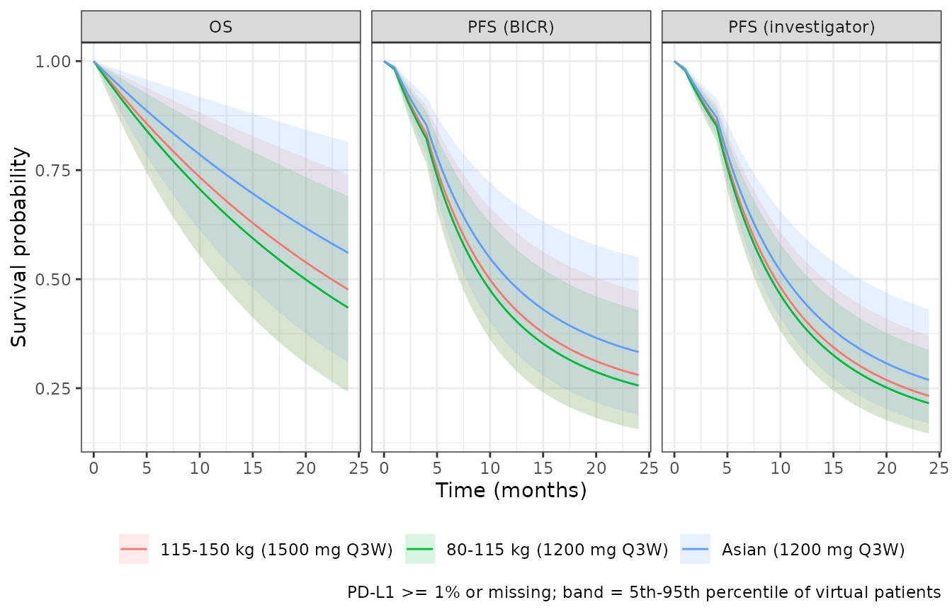
Replicates Figure 3 of Sheng 2026. The bands are narrower than the paper’s because they hold only between-patient exposure variability; the paper’s 90% prediction intervals also include ER parameter uncertainty.
External validation regimen (Figure 1b)
The paper validated the popPK model externally on 13 Asian patients with colorectal cancer (41-95 kg) who received 1800 mg every 4 weeks. The observed data are not public; this plot shows the model’s prediction interval for that regimen over three cycles, for comparison with Figure 1b.
n_ext <- 100
cov_ext <- draw_covariates(n_ext, runif(n_ext, 41, 95), "nsclc") |>
  mutate(TUMTP_NSCLC = 0L)
obs_ext <- sort(c(seq(0, 84, by = 1), 1 / 24, 28 + 1 / 24, 56 + 1 / 24))
ev_ext <- bind_rows(
  make_events(cov_ext, 1800, obs_ext),
  make_events(cov_ext, 1800, 0) |> filter(evid == 1) |> mutate(time = 28),
  make_events(cov_ext, 1800, 0) |> filter(evid == 1) |> mutate(time = 56)
) |>
  arrange(id, time, desc(evid))
sim_ext <- rxode2::rxSolve(mod_pk, ev_ext, returnType = "data.frame")

sim_ext |>
  group_by(time) |>
  summarise(median = median(sim), lo = quantile(sim, 0.05), hi = quantile(sim, 0.95)) |>
  ggplot(aes(time, median)) +
  geom_ribbon(aes(ymin = lo, ymax = hi), alpha = 0.2) +
  geom_line() +
  scale_y_log10() +
  labs(x = "Time (days)", y = "Sugemalimab (ug/mL)", caption = "Median and 90% prediction interval, other solid tumour, 1800 mg Q4W") +
  theme_bw()
#> Warning in scale_y_log10(): log-10 transformation introduced infinite values.
#> log-10 transformation introduced infinite values.
#> log-10 transformation introduced infinite values.
#> log-10 transformation introduced infinite values.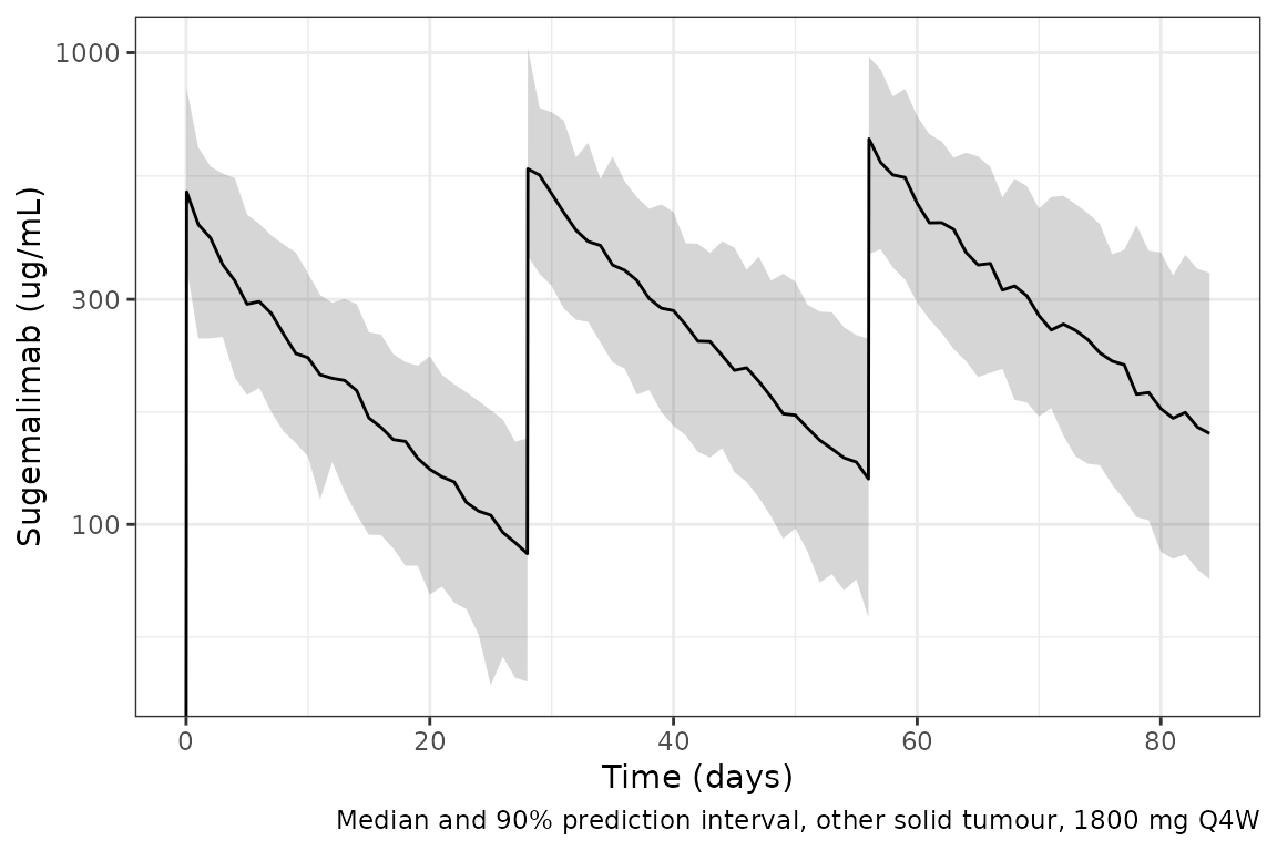
Assumptions and deviations
-
Between-subject variability as SD. Table S2 reports
BSV as percentages. The control stream estimates each SD directly as a
THETA(Cholesky reparameterisation with the OMEGA block fixed to the identity), and the residual error row (16.9) is plainlyTHETA(7)x 100. The BSV rows were therefore read as SD x 100, so the variance is (value / 100)^2 (for example 1.042^2 = 1.086 for Kdes). The same reporting convention is documented in the sugemalimab model of Wang 2024, which shares three authors (Sheng, Xu and Wang K). - Correlations. Only the three correlations that Table S2 reports were estimated; the control stream fixes all others to zero, and they are carried as zero.
-
ADA titre coding. ADA-negative records carry
ADA_TITER = 0.5, half the lowest dilution factor (control stream comment). A value of 0 is undefined in the model. All simulations here are ADA-negative, as in the paper. -
Tumour-type indicators. The source column
DSSTATis 1 for lymphoma and 2 or more for stage III and IV NSCLC; other solid tumours are the remaining level. This is encoded withTUMTP_LYMPH(Kdes and Vc) andTUMTP_NSCLC(Vp). -
Lymphoma Kdes. Table S2 lists “Effect of Lymphoma
Disease on Kdes” as 0.0465, and the control stream replaces the typical
Kdes with this value for lymphoma rather than multiplying it, so it is
carried as a separate typical value
lcl_exp_kdes_lymph. -
Time units. The NONMEM data set is in hours, with
the clearance
THETAs divided by 24; the reported values are per day and the packaged model runs in days. The ER models run in months, as fitted. -
PD-L1 coding. The PFS models raise the hazard for
PD-L1 < 1%; patients with a missing PD-L1 result were grouped with
PD-L1 >= 1%, so they should be supplied as
PDL1_TUM_POS = 1. -
ER exposure is a covariate. The ER models take
CTROUGHas a data column. In the paper it is each patient’s empirical-Bayes prediction from the popPK model; here it is simulated from the popPK model. - Virtual cohorts. The GEMSTONE-302 weight SD (11.7 kg), its female fraction and its albumin distribution are not reported; the Table S1 values of the whole modelling population are used. The infusion duration is not reported; 1 hour is assumed. The GEMSTONE-302 PD-L1 distribution is not reported, so survival is shown per PD-L1 stratum.
- Absolute Table 2 ratios. The geometric-mean ratios of Table 2 are relative to model-predicted GEMSTONE-302 exposures that are not published, so only their dependence on weight and dose is compared.
- External validation. The 1800 mg Q4W colorectal-cancer patients were coded as other solid tumours; their observed concentrations are not public.