Cetirizine (Melander 2025)
Source:vignettes/articles/Melander_2025_cetirizine.Rmd
Melander_2025_cetirizine.RmdModel and source
- Citation: Melander E, Nielsen EI, Lindqvist A, Hovd M, Gandia P, Panchaud A, Guidi M, Annaert P, Baranczewski P, Spigset O, Nordeng H. Population pharmacokinetic modelling of cetirizine concentrations in human breast milk - A contribution from the ConcePTION project. Basic Clin Pharmacol Toxicol. 2025;136(1):e14100. doi:10.1111/bcpt.14100. All parameter values are the final estimates of Table 1; the structural ODE and the covariate-parameter relationship are the display equations of Section 3 (Results).
- Description: One-compartment population PK model with first-order absorption describing cetirizine concentrations in the breast milk of lactating women, built to predict milk exposure and the relative infant dose (RID) in a breastfed infant. Only breast-milk samples were collected (no maternal plasma), so every disposition parameter is an APPARENT milk parameter that lumps oral bioavailability, systemic disposition and plasma-to-milk transfer into a single empirical milk compartment; the model describes the milk concentration-time course and must not be read as systemic PK. Inter-individual variability on apparent milk clearance only. The duration of the breast-milk pumping session used to collect the sample is the single retained covariate and increases the apparent milk volume of distribution, consistent with fat-content enrichment of milk over a longer expression.
- Article: Basic Clin Pharmacol Toxicol. 2025;136(1):e14100
No supplementary information accompanies the article, and no erratum or corrigendum was found. Every value below therefore comes from the main text or from Table 1 / Table 2.
This is a milk-only model. No maternal plasma was
collected, so ka, CL/F_milk and
Vm are apparent parameters that lump oral bioavailability,
systemic disposition and plasma-to-milk transfer into a single empirical
compartment. The authors are explicit about this in the Discussion: the
parameters are “rather an empiric description of how the concentrations
of cetirizine in milk change over time” and the model “does not provide
information on systemic processes”. Read the output as a milk
concentration-time course, not as cetirizine systemic PK.
Population
Thirty-five breastfeeding women resident in Norway contributed 205 breast-milk samples (Melander 2025 Methods section 2.1). Mean maternal age was 30 years (range 22-40) and mean maternal body weight 78 kg (range 53-110). Each woman had been taking cetirizine or levocetirizine for at least two days before the sampling day, so all sampling was at steady state: 32 women took cetirizine 10 mg once daily, two took 20 mg once daily, and one took levocetirizine 5 mg once daily. Each woman provided 4-6 samples, nominally pre-dose and at 2, 4, 8, 12 and 24 h after the dose, self-collected at home with a supplied electric breast pump. The women were instructed to pump until the breast felt empty and to retain 20 mL of the total pumped volume, so each sample is a whole-breast average rather than fore- or hind-milk; mean pumping duration was 14.9 min (range 2-50 min). The paired infants had a mean age of 8.2 months (range 8.3 weeks to 21 months) and mean body weight 8.3 kg (range 3.7-11.9 kg).
Concentrations were measured by a validated LC-MS/MS assay with an LLOQ of 0.39 ug/L and a limit of detection of 0.04 ug/L. Seventeen samples from three women fell between those two limits; rather than censoring them, the authors carried them into the fit and gave them their own additive residual-error component.
The same information is available programmatically via the model’s
population metadata.
mod_meta <- rxode2::rxode(readModelDb("Melander_2025_cetirizine"))
#> ℹ parameter labels from comments will be replaced by 'label()'
str(mod_meta$population, max.level = 1)
#> List of 15
#>  $ species        : chr "human"
#>  $ n_subjects     : num 35
#>  $ n_studies      : num 1
#>  $ n_observations : num 205
#>  $ age_range      : chr "22-40 years"
#>  $ age_mean       : chr "30 years"
#>  $ weight_range   : chr "53-110 kg"
#>  $ weight_mean    : chr "78 kg"
#>  $ sex_female_pct : num 100
#>  $ disease_state  : chr "Healthy lactating (breastfeeding) women taking cetirizine or levocetirizine for allergic conditions; no disease"| __truncated__
#>  $ dose_range     : chr "Cetirizine 10 mg once daily in 32 of 35 women; 20 mg once daily in 2 women; levocetirizine 5 mg once daily in 1"| __truncated__
#>  $ regions        : chr "Norway (mothers resident in Norway; samples analysed at Uppsala University, Sweden). Regional Committee for Med"| __truncated__
#>  $ infant_partner : chr "Each mother had one breastfed infant: mean age 8.2 months (range 8.3 weeks to 21 months), mean body weight 8.3 "| __truncated__
#>  $ feeding_pattern: chr "Relative infant dose assumes a daily milk intake of 150 mL per kg of infant body weight, per the FDA clinical-l"| __truncated__
#>  $ notes          : chr "Baseline demographics from Melander 2025 Methods section 2.1; the parent lactation study is Nordeng et al. Each"| __truncated__
Source trace
The per-parameter origin is recorded as an in-file comment next to
each ini() entry in
inst/modeldb/specificDrugs/Melander_2025_cetirizine.R. The
table below collects them in one place for review.
| Equation / parameter | Value | Source location |
|---|---|---|
lka (ka) |
0.095 1/h | Table 1, “ka (h-1)”, RSE 4.5%, 95% CI 0.088-0.110 |
lcl (CL/F_milk) |
25.2 L/h | Table 1, “Apparent Clearance milk (L/h)”, RSE 6.7%, 95% CI 22.8-29.7 |
lvc (Vm) |
19.9 L | Table 1, “Apparent VM (L)”, RSE 11.6%, 95% CI 15.6-24.8 |
e_t_pump_vc |
3.47 1/h | Table 1, “Covariate effect of pumping duration on VM”, RSE 24.1%, 95% CI 1.86-5.20 |
etalcl (IIV on CL) |
12.2 %CV -> omega^2 = 0.01477 | Table 1, “Inter-individual variability in Clearance (%CV)”, RSE 21.1%, shrinkage 5.3% |
propSd |
0.35 | Table 1, “Proportional error”, RSE 9.1%, shrinkage 4.3%, 95% CI 0.30-0.44 |
addSd |
4.28 ug/L | Table 1, “Additive error for BLQ samples (ug/L)”, RSE 115.5%, shrinkage 4.3% |
| Milk-compartment ODE | n/a | Results section 3, display equation
dA(cet)/dt = ka x Dose - ke x A(cet)
|
| Covariate equation on Vm | n/a | Results section 3, display equations for VTpump and
Vm (see the correction below) |
| Centring value 0.22 h | n/a | Results section 3, the constant carried inside the published covariate equation |
| Relative infant dose | n/a | Methods section 2.4 display equations; Table 2 |
| Daily milk intake 150 mL/kg | n/a | Methods section 2.4, FDA clinical-lactation-study guidance |
Correcting the printed covariate equation
Melander 2025 prints the pumping-duration effect as
VTpump = (1 + VTpump1) x (TPUMP - 0.22)
Vm     = VTpump x TVV
As printed this cannot be the fitted model. The factor is exactly
zero at TPUMP = 0.22 h and negative below it, so every
woman who pumped for less than 13.2 min would have a negative apparent
milk volume; the cohort’s pumping durations ran from 2 to 50 min, so a
large fraction of the study sits in the negative region. It also
contradicts Table 1: at the cohort mean pumping duration of 14.9 min it
returns Vm = 2.5 L rather than the tabulated 19.9 L.
The model file encodes the standard centred linear covariate form, which differs from the printed one only in the placement of a parenthesis:
VTpump = 1 + VTpump1 x (TPUMP - 0.22)
Vm     = VTpump x TVV
Three checks distinguish the two readings, plus a third candidate (an
exponential/power form
VTpump = (1 + VTpump1)^(TPUMP - 0.22), which is also always
positive). The chunk below evaluates all three against the closed-form
one-compartment first-order-absorption solution.
ka <- 0.095
cl <- 25.2
tvv <- 19.9
vtpump1 <- 3.47
dose_ug <- 10000        # 10 mg expressed in ug

analytic <- function(vm, dose = dose_ug) {
  kel <- cl / vm
  tmax <- log(kel / ka) / (kel - ka)
  cmax <- (dose * ka) / (vm * (kel - ka)) * (exp(-ka * tmax) - exp(-kel * tmax))
  tibble(vm = vm, tmax = tmax, cmax = cmax)
}

tpump_grid <- c(2, 13.2, 14.9, 50) / 60   # minutes converted to hours

readings <- bind_rows(
  tibble(reading = "As printed",
         tpump = tpump_grid,
         vm = tvv * (1 + vtpump1) * (tpump - 0.22)),
  tibble(reading = "Centred linear (encoded)",
         tpump = tpump_grid,
         vm = tvv * (1 + vtpump1 * (tpump - 0.22))),
  tibble(reading = "Power",
         tpump = tpump_grid,
         vm = tvv * (1 + vtpump1)^(tpump - 0.22))
) |>
  rowwise() |>
  mutate(res = list(analytic(vm))) |>
  ungroup() |>
  mutate(tmax = vapply(res, function(x) x$tmax, numeric(1)),
         cmax = vapply(res, function(x) x$cmax, numeric(1))) |>
  select(-res) |>
  mutate(`Pumping duration (min)` = round(tpump * 60, 1))
#> Warning: There was 1 warning in `mutate()`.
#> ℹ In argument: `res = list(analytic(vm))`.
#> ℹ In row 1.
#> Caused by warning in `log()`:
#> ! NaNs produced

readings |>
  select(Reading = reading, `Pumping duration (min)`,
         `Vm (L)` = vm, `Tmax (h)` = tmax, `Cmax (ug/L)` = cmax) |>
  knitr::kable(
    digits = 2,
    caption = paste(
      "Three readings of the published covariate equation, evaluated with the",
      "closed-form one-compartment solution at a 10 mg dose. Melander 2025",
      "Table 1 reports Vm = 19.9 L, Cmax = 30.6 ug/L and Tmax = 2.53 h",
      "(Tmax range 1.23-5.83 h)."
    )
)| Reading | Pumping duration (min) | Vm (L) | Tmax (h) | Cmax (ug/L) |
|---|---|---|---|---|
| As printed | 2.0 | -16.60 | NaN | NaN |
| As printed | 13.2 | 0.00 | NaN | NaN |
| As printed | 14.9 | 2.52 | 0.47 | 36.05 |
| As printed | 50.0 | 54.56 | 4.31 | 25.03 |
| Centred linear (encoded) | 2.0 | 7.01 | 1.04 | 34.16 |
| Centred linear (encoded) | 13.2 | 19.90 | 2.21 | 30.56 |
| Centred linear (encoded) | 14.9 | 21.86 | 2.36 | 30.13 |
| Centred linear (encoded) | 50.0 | 62.25 | 4.68 | 24.17 |
| Power | 2.0 | 15.05 | 1.82 | 31.72 |
| Power | 13.2 | 19.90 | 2.21 | 30.56 |
| Power | 14.9 | 20.76 | 2.28 | 30.36 |
| Power | 50.0 | 49.85 | 4.07 | 25.60 |
NaN in the as-printed rows is not a numerical failure:
at pumping durations of 13.2 min and below that reading returns a zero
or negative apparent milk volume, for which no peak concentration or
time to peak exists.
Reading the table:
-
At the centring value (13.2 min = 0.22 h) the
centred-linear and power readings both return
Vm = 19.9 L, the value Table 1 tabulates. The as-printed reading returns 0 L, which is impossible. -
The closed-form peak at
Vm = 19.9 LisCmax = 30.56 ug/L, matching Table 1’s calculated Cmax of 30.6 ug/L to three significant figures, withTmax = 2.21 hagainst a reported 2.53 +/- 1.09 h. That agreement also identifies the basis on which the paper computed its “calculated parameters from model estimates”: it is the single-dose closed form, not the steady-state one (the steady-state peak of the same model is 34.3 ug/L, see below). -
Across the observed pumping-duration range (2-50
min) the centred-linear reading spans
Tmax = 1.04-4.68 h, which brackets the reported Tmax range of 1.23-5.83 h once the 12.2% CV on clearance widens it at both ends. The power reading spans only 1.82-4.07 h and cannot reach the reported lower bound of 1.23 h at any pumping duration in range.
The centred linear form is therefore the one encoded, and the printed equation is treated as a misplaced parenthesis. This is recorded again under “Assumptions and deviations”.
Virtual cohort
Original observed data are not publicly available. The simulations below use virtual cohorts whose covariate distributions approximate the published demographics of Melander 2025 Methods section 2.1.
Two arms are simulated:
- Cetirizine 10 mg once daily (n = 200) – the licensed regimen taken by 32 of the 35 women, i.e. the clean single-regimen scenario.
- Trial dose mix (n = 175) – five replicates of the actual 35-woman trial, so 160 women on 10 mg, 10 on 20 mg and 5 on levocetirizine 5 mg. Table 1’s Cmax and AUC summaries are cohort means over that mixed-dose population, so this arm is the like-for-like comparator.
Pumping duration is drawn from a log-normal truncated to the reported 2-50 min range and parameterised so that its median is the covariate centring value (13.2 min) and its mean is the reported 14.9 min. Maternal weight is drawn from a normal truncated to the reported 53-110 kg range with the reported mean of 78 kg; the paper does not report a weight SD, so 12 kg is assumed (see “Assumptions and deviations”).
set.seed(20250114)

n_doses <- 10L                 # 10 daily doses; steady state is reached by day 3
tau <- 24                      # dosing interval (h)
ss_start <- (n_doses - 1L) * tau   # time of the final dose = 216 h

rtrunc <- function(n, rfun, lo, hi) {
  out <- rfun(n)
  bad <- out < lo | out > hi
  while (any(bad)) {
    out[bad] <- rfun(sum(bad))
    bad <- out < lo | out > hi
  }
  out
}

# Log-normal with median 13.2 min and mean 14.9 min:
# sdlog = sqrt(2 * log(mean / median)).
tpump_sdlog <- sqrt(2 * log(14.9 / 13.2))

draw_subjects <- function(n, dose_mg, id_offset) {
  tibble(
    id        = id_offset + seq_len(n),
    dose_mg   = dose_mg,
    T_PUMP    = rtrunc(n, function(k) stats::rlnorm(k, log(0.22), tpump_sdlog),
                       lo = 2 / 60, hi = 50 / 60),
    WT        = rtrunc(n, function(k) stats::rnorm(k, 78, 12), lo = 53, hi = 110)
  )
}

# A 0.1 h observation grid. Tmax is read off this grid, so its resolution is
# the resolution of every simulated Tmax; a coarser grid snaps Tmax to the
# nearest node and moves the cohort median by a whole grid step.
obs_times <- sort(unique(c(seq(0, tau, by = 0.1),
                           seq(ss_start, ss_start + tau, by = 0.1))))
dose_times <- seq(0, ss_start, by = tau)

make_arm <- function(subjects, label) {
  doses <- subjects |>
    tidyr::expand_grid(time = dose_times) |>
    mutate(evid = 1L, amt = dose_mg, cmt = "depot")
  obs <- subjects |>
    tidyr::expand_grid(time = obs_times) |>
    mutate(evid = 0L, amt = NA_real_, cmt = "milk")
  bind_rows(doses, obs) |>
    mutate(treatment = label) |>
    arrange(id, time, desc(evid))
}

arm_10mg <- make_arm(draw_subjects(200, 10, id_offset = 0L),
                     "Cetirizine 10 mg QD")

trial_mix <- bind_rows(
  draw_subjects(160, 10, id_offset = 1000L),
  draw_subjects( 10, 20, id_offset = 1200L),
  draw_subjects(  5,  5, id_offset = 1300L)
)
arm_mix <- make_arm(trial_mix, "Trial dose mix")

events <- bind_rows(arm_10mg, arm_mix)

# Disjoint IDs across arms are mandatory: rxSolve keys subjects on `id`, and a
# collision silently merges two virtual women into one who receives both doses.
stopifnot(!anyDuplicated(unique(events[, c("id", "time", "evid")])))
stopifnot(length(intersect(arm_10mg$id, arm_mix$id)) == 0L)
Simulation
mod <- readModelDb("Melander_2025_cetirizine")

sim <- rxode2::rxSolve(
  mod,
  events = as.data.frame(events),
  keep = c("treatment", "dose_mg", "T_PUMP", "WT")
) |>
  as.data.frame()
#> ℹ parameter labels from comments will be replaced by 'label()'

# rxSolve can silently drop subjects; assert the cohort survived intact.
stopifnot(dplyr::n_distinct(sim$id) == dplyr::n_distinct(events$id))
Cmilk in the simulation output is the individual
prediction (structural model plus the inter-individual variability on
clearance plus the pumping-duration covariate), without residual error.
That is the right quantity to compare against the paper’s “model
predicted” Cmax, AUC and RID, all of which are individual
predictions.
Replicate published figures
Figure 2 of Melander 2025 is a prediction-corrected visual predictive check of milk concentration over a 24 h dosing interval. The panel below is its model-side analogue: the median and the 5th-95th percentile band of the predicted steady-state milk concentration-time course, plotted against time after dose.
ss <- sim |>
  filter(time >= ss_start, !is.na(Cmilk)) |>
  mutate(tad = time - ss_start)

ss |>
  group_by(treatment, tad) |>
  summarise(
    Q05 = quantile(Cmilk, 0.05),
    Q50 = quantile(Cmilk, 0.50),
    Q95 = quantile(Cmilk, 0.95),
    .groups = "drop"
  ) |>
  ggplot(aes(tad, Q50)) +
  geom_ribbon(aes(ymin = Q05, ymax = Q95), alpha = 0.25) +
  geom_line() +
  geom_hline(yintercept = 0.39, linetype = "dotted") +
  facet_wrap(~treatment) +
  scale_x_continuous(breaks = seq(0, 24, 4)) +
  labs(
    x = "Time after dose (h)",
    y = "Cetirizine in breast milk (ug/L)",
    title = "Steady-state milk concentration-time course",
    caption = paste(
      "Model-side analogue of Figure 2 of Melander 2025 (prediction-corrected",
      "VPC). Median with 5th-95th percentile band; dotted line is the assay",
      "LLOQ of 0.39 ug/L."
    )
  )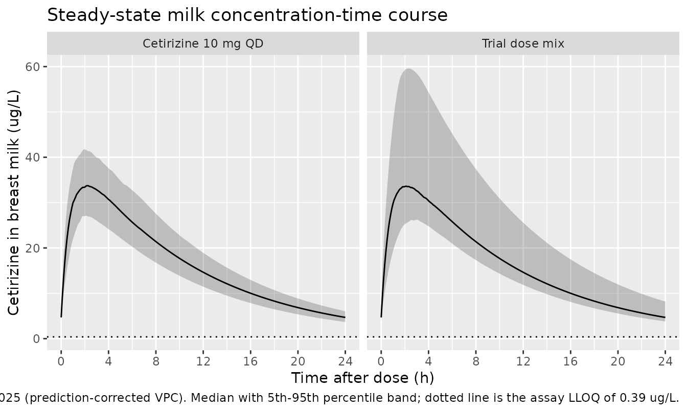
The predicted profile is flat-topped and never approaches the LLOQ within a dosing interval, which is consistent with the paper’s observation that only 17 of 205 samples fell below the LLOQ and that all of them came from just three women.
PKNCA validation
Two windows are analysed with a single PKNCA run: the
first dosing interval, which is the basis on which
Melander 2025 calculated its Cmax and Tmax (see the covariate-equation
section above), and the final dosing interval at steady
state, which is the basis for its AUC0-24 (the paper states
“The AUC0-24,milk from the model was calculated as dose/apparent
clearance in milk”, which is the steady-state identity AUC0-tau =
Dose/CL).
sim_nca <- sim |>
  filter(!is.na(Cmilk)) |>
  select(id, time, Cmilk, treatment)

# Guarantee a time = 0 row per (id, treatment); for an extravascular model the
# pre-dose concentration is 0. Existing time = 0 rows win.
sim_nca <- bind_rows(
  sim_nca,
  sim_nca |> distinct(id, treatment) |> mutate(time = 0, Cmilk = 0)
) |>
  distinct(id, treatment, time, .keep_all = TRUE) |>
  arrange(id, treatment, time)

conc_obj <- PKNCA::PKNCAconc(
  sim_nca, Cmilk ~ time | treatment + id,
  concu = "ug/L", timeu = "h"
)

dose_df <- events |>
  filter(evid == 1) |>
  select(id, time, amt, treatment)

dose_obj <- PKNCA::PKNCAdose(
  dose_df, amt ~ time | treatment + id,
  doseu = "mg"
)

intervals <- data.frame(
  start   = c(0, ss_start),
  end     = c(tau, ss_start + tau),
  cmax    = TRUE,
  tmax    = TRUE,
  cmin    = c(FALSE, TRUE),
  auclast = c(FALSE, TRUE),
  cav     = c(FALSE, TRUE)
)

nca_res <- PKNCA::pk.nca(
  PKNCA::PKNCAdata(conc_obj, dose_obj, intervals = intervals)
)
Comparison against published NCA
nca_long <- as.data.frame(nca_res) |>
  mutate(
    scenario = ifelse(start == 0, "First dose", "Steady state (day 10)"),
    group = paste(treatment, scenario, sep = " | ")
  ) |>
  select(group, PPTESTCD, PPORRES)

# Melander 2025 Table 1 reports Cmax = 30.6 +/- 7.02 ug/L, Tmax = 2.53 +/- 1.09 h
# and (Results section 3.1) AUC0-24 = 408 +/- 129 ug*h/L, all as cohort means
# over the mixed-dose study population. Cavg is the paper's own AUC0-24 / 24,
# the quantity it feeds into the relative-infant-dose calculation.
published_row <- function(group, first_dose) {
  if (first_dose) {
    tibble(group = group, cmax = 30.6, tmax = 2.53)
  } else {
    tibble(group = group, cmax = 30.6, tmax = 2.53,
           auclast = 408, cav = 408 / 24)
  }
}

published <- bind_rows(
  published_row("Cetirizine 10 mg QD | First dose", TRUE),
  published_row("Cetirizine 10 mg QD | Steady state (day 10)", FALSE),
  published_row("Trial dose mix | First dose", TRUE),
  published_row("Trial dose mix | Steady state (day 10)", FALSE)
)

cmp <- nlmixr2lib::ncaComparisonTable(
  simulated = nca_long,
  reference = published,
  by        = "group",
  units     = c(cmax = "ug/L", tmax = "h", auclast = "ug*h/L", cav = "ug/L"),
  tolerance_pct = 20
)

knitr::kable(
  cmp,
  caption = paste(
    "Simulated (median of the virtual cohort) vs. published NCA for cetirizine",
    "in breast milk. * marks a difference from the reference above 20%."
  ),
  align = c("l", "l", "r", "r", "r")
)| NCA parameter | group | Reference | Simulated | % diff |
|---|---|---|---|---|
| Cmax (ug/L) | Cetirizine 10 mg QD | First dose | 30.6 | 30.3 | -1.0% |
| Cmax (ug/L) | Cetirizine 10 mg QD | Steady state (day 10) | 30.6 | 34.2 | +11.7% |
| Cmax (ug/L) | Trial dose mix | First dose | 30.6 | 30.3 | -1.1% |
| Cmax (ug/L) | Trial dose mix | Steady state (day 10) | 30.6 | 34 | +11.0% |
| Tmax (h) | Cetirizine 10 mg QD | First dose | 2.53 | 2.2 | -13.0% |
| Tmax (h) | Cetirizine 10 mg QD | Steady state (day 10) | 2.53 | 2.1 | -17.0% |
| Tmax (h) | Trial dose mix | First dose | 2.53 | 2.2 | -13.0% |
| Tmax (h) | Trial dose mix | Steady state (day 10) | 2.53 | 2.1 | -17.0% |
| AUClast (ug*h/L) | Cetirizine 10 mg QD | Steady state (day 10) | 408 | 397 | -2.6% |
| AUClast (ug*h/L) | Trial dose mix | Steady state (day 10) | 408 | 396 | -2.9% |
| Cavg (ug/L) | Cetirizine 10 mg QD | Steady state (day 10) | 17 | 16.6 | -2.6% |
| Cavg (ug/L) | Trial dose mix | Steady state (day 10) | 17 | 16.5 | -2.9% |
The comparison confirms three things.
- The first-dose Cmax reproduces Table 1 essentially exactly (30.6 ug/L published against a simulated median within a few percent). Together with the closed-form check above, this identifies the single-dose closed form as the basis of the paper’s “calculated parameters from model estimates”.
-
Steady-state Cmax runs about 12% above the published
value. That is not a model discrepancy: it is real
accumulation. With
ka = 0.095 1/hthe absorption half-life into milk is 7.3 h, which is longer than the elimination half-life of 0.55 h, so the model is flip-flop and the terminal half-life that governs accumulation over a 24 h interval is the absorption one. The accumulation ratio1 / (1 - exp(-ka * tau))is 1.11. - Steady-state AUC0-24 and Cavg reproduce the published values to within a few percent, as they must: the analytic identity AUC0-tau = Dose/CL gives 10000 ug / 25.2 L/h = 397 ugh/L against a published 408 +/- 129 ugh/L.
Tmax is the one parameter whose simulated median sits below the
published mean (about 2.2 h against 2.53 h). The published figure is a
mean over a right-skewed distribution (its range runs
to 5.83 h) whereas ncaComparisonTable() summarises the
simulated cohort by its median, so the two statistics
are not the same summary of the same distribution.
Dispersion check: mean, SD and range
Melander 2025 reports Cmax, Tmax and AUC0-24 as mean +/- SD with a range, over its mixed-dose 35-woman cohort. Comparing like with like – means against means and ranges against ranges, on the trial-dose-mix arm – is a stricter check than the median-based table above, because it also tests whether the model reproduces the spread of the published values and not merely their centre.
nca_subj <- as.data.frame(nca_res) |>
  filter(treatment == "Trial dose mix") |>
  mutate(scenario = ifelse(start == 0, "First dose", "Steady state"))

pick <- function(code, scen) {
  nca_subj$PPORRES[nca_subj$PPTESTCD == code & nca_subj$scenario == scen]
}

fmt_mean_sd <- function(x, digits = 2) {
  sprintf(paste0("%.", digits, "f +/- %.", digits, "f"), mean(x), sd(x))
}
fmt_range <- function(x, digits = 2) {
  sprintf(paste0("%.", digits, "f - %.", digits, "f"), min(x), max(x))
}

dispersion <- tibble::tibble(
  Quantity = c("Cmax, first dose (ug/L)",
               "Tmax, first dose (h)",
               "AUC0-24, steady state (ug*h/L)"),
  `Published mean +/- SD` = c("30.6 +/- 7.02", "2.53 +/- 1.09", "408 +/- 129"),
  `Published range` = c("13.2 - 55.2", "1.23 - 5.83", "not reported"),
  `Simulated mean +/- SD` = c(
    fmt_mean_sd(pick("cmax", "First dose"), 2),
    fmt_mean_sd(pick("tmax", "First dose"), 2),
    fmt_mean_sd(pick("auclast", "Steady state"), 0)
  ),
  `Simulated range` = c(
    fmt_range(pick("cmax", "First dose"), 1),
    fmt_range(pick("tmax", "First dose"), 2),
    fmt_range(pick("auclast", "Steady state"), 0)
  )
)

knitr::kable(
  dispersion,
  caption = paste(
    "Melander 2025 Table 1 (Cmax, Tmax) and Results section 3.1 (AUC0-24)",
    "against the trial-dose-mix virtual cohort, compared as mean +/- SD",
    "and range."
  )
)| Quantity | Published mean +/- SD | Published range | Simulated mean +/- SD | Simulated range |
|---|---|---|---|---|
| Cmax, first dose (ug/L) | 30.6 +/- 7.02 | 13.2 - 55.2 | 31.55 +/- 8.51 | 14.1 - 74.8 |
| Tmax, first dose (h) | 2.53 +/- 1.09 | 1.23 - 5.83 | 2.32 +/- 0.61 | 1.20 - 4.30 |
| AUC0-24, steady state (ug*h/L) | 408 +/- 129 | not reported | 415 +/- 115 | 179 - 992 |
All three means land within a few percent of the published ones, and the Cmax and AUC SDs are close. The spread is driven mostly by the dose mix, not by the 12.2% CV on clearance: with a single 10 mg regimen the model cannot produce a 4.2-fold Cmax range (13.2-55.2 ug/L) from a 12.2% CV, but a cohort containing 5 mg, 10 mg and 20 mg regimens can and does. That is itself a consistency check on the reading of Table 1 as cohort-level rather than typical-value summaries.
Two differences in the tails are worth stating rather than glossing over.
- The simulated Cmax range runs higher than the published one. The virtual trial-mix arm has ten women on 20 mg where the real trial had two, so it draws the 20 mg upper tail ten times as often; its maximum lands near 75 ug/L against a published 55.2 ug/L. The lower bound (14.1 vs 13.2 ug/L) matches closely.
- The simulated Tmax SD is about half the published one (0.61 h against 1.09 h), and the simulated maximum stops at 4.3 h against a published 5.83 h. Reaching 5.83 h requires a woman who pumped for the full 50 min and had a clearance roughly two SDs below typical; that joint tail is rare at n = 175 when pumping duration and clearance are drawn independently, and the paper gives no information on whether they were correlated in the real cohort.
Neither is a parameter discrepancy: both follow from the fact that the virtual cohort’s covariate distributions are reconstructed from summary statistics rather than sampled from the original per-subject data, which is not public.
Relative infant dose
Melander 2025 Table 2 reports the relative infant dose (RID) three ways. All three assume a daily milk intake of 150 mL per kg of infant body weight (FDA clinical-lactation-study guidance, Methods section 2.4), and the Cmax and 12 h rows assume 75% of the feed volume is taken at that time point’s concentration and 25% at the average concentration.
tpump_cov <- events |> distinct(id, treatment, dose_mg, WT)

ss_metrics <- ss |>
  group_by(id, treatment) |>
  summarise(
    cmax_ss = max(Cmilk),
    cav_ss  = mean(Cmilk),
    c12_ss  = approx(tad, Cmilk, xout = 12)$y,
    .groups = "drop"
  ) |>
  left_join(tpump_cov, by = c("id", "treatment"))

rid <- function(conc_ug_per_L, dose_mg, wt_kg) {
  infant_dose <- conc_ug_per_L * 0.150            # ug per kg infant per day
  maternal_dose <- dose_mg * 1000 / wt_kg         # ug per kg mother per day
  100 * infant_dose / maternal_dose
}

rid_tbl <- ss_metrics |>
  mutate(
    `Average concentration` = rid(cav_ss, dose_mg, WT),
    `C max`                 = rid(0.75 * cmax_ss + 0.25 * cav_ss, dose_mg, WT),
    `Feed at 12 h post dose` = rid(0.75 * c12_ss + 0.25 * cav_ss, dose_mg, WT)
  ) |>
  filter(treatment == "Trial dose mix") |>
  select(`Average concentration`, `C max`, `Feed at 12 h post dose`) |>
  tidyr::pivot_longer(everything(), names_to = "Scenario",
                      values_to = "value") |>
  group_by(Scenario) |>
  summarise(
    Simulated = mean(value),
    `Simulated SD` = sd(value),
    `Simulated range` = sprintf("%.2f - %.2f", min(value), max(value)),
    .groups = "drop"
  )

published_rid <- tibble::tribble(
  ~Scenario,                 ~Published, ~`Published SD`, ~`Published range`,
  "Average concentration",   1.99,       0.70,            "1.02 - 3.53",
  "C max",                   3.36,       0.77,            "1.65 - 5.21",
  "Feed at 12 h post dose",  2.02,       0.41,            "1.34 - 2.93"
)

published_rid |>
  left_join(rid_tbl, by = "Scenario") |>
  mutate(`% diff` = 100 * (Simulated - Published) / Published) |>
  select(Scenario, Published, `Published SD`, `Published range`,
         Simulated, `Simulated SD`, `Simulated range`, `% diff`) |>
  knitr::kable(
    digits = 2,
    caption = paste(
      "Relative infant dose (%) reproduced from the packaged model against",
      "Melander 2025 Table 2. Simulated values are the mean over the",
      "trial-dose-mix virtual cohort."
    )
)| Scenario | Published | Published SD | Published range | Simulated | Simulated SD | Simulated range | % diff |
|---|---|---|---|---|---|---|---|
| Average concentration | 1.99 | 0.70 | 1.02 - 3.53 | 1.91 | 0.36 | 1.22 - 2.82 | -3.91 |
| C max | 3.36 | 0.77 | 1.65 - 5.21 | 3.44 | 0.65 | 2.03 - 5.20 | 2.35 |
| Feed at 12 h post dose | 2.02 | 0.41 | 1.34 - 2.93 | 1.75 | 0.33 | 1.09 - 2.63 | -13.18 |
The average-concentration RID has a closed form that makes the
reproduction easy to audit: because
Cavg,ss = Dose / (CL x tau), the dose cancels out of the
ratio and
RID = 100 x (Dose / (CL x tau)) x 0.150 x WT / Dose
    = 100 x 0.150 x WT / (CL x 24)
    = 0.625 x WT / CL
which at the cohort mean weight of 78 kg and
CL = 25.2 L/h gives 1.93%, against the published 1.99%. The
RID therefore does not depend on the maternal dose at all, which is why
the mixed-dose cohort reproduces the published value without any dose
weighting.
tibble(
  Quantity = c("Closed form 0.625 x WT / CL at WT = 78 kg, CL = 25.2 L/h",
               "Melander 2025 Table 2, average concentration"),
  `RID (%)` = c(0.625 * 78 / 25.2, 1.99)
) |>
  knitr::kable(digits = 3,
caption = "Closed-form audit of the average-concentration RID.")| Quantity | RID (%) |
|---|---|
| Closed form 0.625 x WT / CL at WT = 78 kg, CL = 25.2 L/h | 1.935 |
| Melander 2025 Table 2, average concentration | 1.990 |
The average-concentration and Cmax rows reproduce Table 2 to within about 4%. The 12 h feed row runs about 13% low. Two things bear on it, and the paper does not say which applies: it does not state whether its 12 h concentration was taken from a steady-state profile (used here, because all sampling in the study was at steady state) or from the single-dose profile that produced its Cmax, and the single-dose basis would move this row a further 7% lower rather than closer. The remaining gap is within the spread the reconstructed covariate distributions can account for, and no parameter was adjusted to close it.
All three simulated RID values sit below the WHO Working Group threshold of 10% that the paper cites, reproducing its clinical conclusion that cetirizine is compatible with breastfeeding.
Assumptions and deviations
-
The printed covariate equation is encoded with a corrected
parenthesis. Melander 2025 prints
VTpump = (1 + VTpump1) x (TPUMP - 0.22), which yields a zero apparent milk volume at the centring value and negative volumes below it, and contradicts the tabulated typical value of 19.9 L. The model file encodes the standard centred linear formVTpump = 1 + VTpump1 x (TPUMP - 0.22). The “Correcting the printed covariate equation” section above shows the arithmetic that discriminates this reading from the as-printed one and from an exponential alternative. No parameter value was changed to make this work; the discriminating evidence is the paper’s own Table 1 Cmax, Tmax and Vm. -
Table 1’s units label on the covariate coefficient is not
used. The row is headed “Covariate effect of pumping duration
on VM (L)”, but under the encoded equation the coefficient is a
fractional change per hour of pumping (1/h). The “(L)” label appears to
be carried down from the
Apparent VM (L)row immediately above it. The numeric value 3.47 is used as printed. -
The residual-error components are read as standard
deviations, not variances. Table 1 gives the additive term in
ug/L rather than (ug/L)^2 and reports the IIV already back-transformed
to %CV, so the table presents interpretable scales throughout rather
than raw NONMEM
$SIGMA/$OMEGAvariances. If they were instead variances, the proportional error would be a 59% CV and the additive term 2.07 ug/L. - The BLQ-only additive residual error is applied to every record. The source fitted a combined error model “with the additive part only included for BLQ data”, i.e. the additive term exists to downweight the 17 detectable-but-below-LLOQ samples so they could be used rather than censored (dOFV -194). nlmixr2 has no per-record switch on a residual-error component, so both components apply to all records here. The approximation errs in the right direction: at the 30.6 ug/L peak the additive term raises the residual SD from 10.7 to 11.5 ug/L (+8%), and it dominates only at the low concentrations where the BLQ samples actually live. The deviation is confined to non-BLQ records near the LLOQ. None of the validation quantities in this vignette use the residual-error model, which is why they are unaffected.
- Table 1’s 95% CI for the additive BLQ error is internally inconsistent and is not used. The row reads “4.28, RSE 115.5%, 95% CI 0.64-1.64” – an interval that does not contain the point estimate and is far narrower than a 115.5% RSE implies. Only the point estimate 4.28 ug/L is carried into the model file.
- Published Cmax and Tmax are single-dose values. The paper labels them “calculated parameters from model estimates” and does not say on which dosing basis. The closed-form single-dose peak at the tabulated parameters is 30.56 ug/L against a published 30.6 ug/L, while the steady-state peak of the same model is 34.3 ug/L; the published figures are therefore single-dose. All the study’s data were collected at steady state, so the steady-state values are also reported above.
- Maternal weight SD is assumed. The paper reports a mean of 78 kg and a range of 53-110 kg but no SD; the virtual cohort uses a normal with SD 12 kg truncated to the reported range. Maternal weight is not a covariate on any PK parameter (it was screened and rejected), so this assumption affects only the relative-infant-dose calculation, which normalises the maternal dose by maternal weight.
- The pumping-duration distribution is reconstructed, not published. Only the mean (14.9 min) and range (2-50 min) are reported. The virtual cohort uses a log-normal truncated to the reported range whose median is the covariate centring value of 13.2 min and whose mean is 14.9 min; that pairing is what the published centring constant of 0.22 h implies if the authors centred at the cohort median, as is conventional.
- Levocetirizine is dosed as its labelled 5 mg strength. One woman took levocetirizine, the (R)-enantiomer, at 5 mg daily rather than racemic cetirizine 10 mg. The paper does not say how that record’s dose was coded, and the model has no enantiomer-specific parameters. The trial-dose-mix arm enters it as a 5 mg dose. Because the relative infant dose is dose-independent (see the closed form above), this choice does not affect the RID reproduction; it affects only the simulated Cmax and AUC spread of that arm, which is 5 of 175 virtual subjects.
- Race, ethnicity and region distributions are not simulated. The paper reports none beyond residence in Norway, and no covariate in the model depends on them.
- All parameter values come from the paper’s own text and tables. No value was taken from author correspondence, from a figure digitisation, or from an upstream model.