GalNAc-conjugated siRNA plasma pharmacokinetics (Sten 2023)
Source:vignettes/articles/Sten_2023_galnacSirna.Rmd
Sten_2023_galnacSirna.RmdModel and source
- Citation: Sten S, Cardilin T, Antonsson M, Gennemark P. Plasma Pharmacokinetics of N-Acetylgalactosamine-Conjugated Small-Interfering Ribonucleic Acids (GalNAc-Conjugated siRNAs). Clin Pharmacokinet. 2023;62(12):1661-1672.
- Article: https://doi.org/10.1007/s40262-023-01314-7 (open access, PMC10684612)
- Original mPBPK-PD model: Ayyar VS et al. J Pharmacol Exp Ther. 2021;379(2):134-146. https://doi.org/10.1124/jpet.121.000805
Sten 2023 pooled published plasma pharmacokinetics of nine GalNAc-conjugated siRNAs and reported four kinds of model. Three of them are ODE models and are packaged here:
| Model file | What it is | Source |
|---|---|---|
Sten_2023_givosiran_che,
Sten_2023_givosiran_aip, Sten_2023_vutrisiran,
Sten_2023_lumasiran_healthy,
Sten_2023_lumasiran_ph1,
Sten_2023_olpasiran_1cmt,
Sten_2023_inclisiran_renalnormal,
Sten_2023_inclisiran_renalmild,
Sten_2023_inclisiran_renalmoderate,
Sten_2023_inclisiran_renalsevere
|
Ten independent one-compartment fits (first-order absorption) to the first 24 or 48 h after dose, one per compound and population | ESM Table S4 |
Sten_2023_olpasiran_3cmt |
Three-compartment fit to olpasiran alone (data to 12 weeks) | Table 3, column 1 |
Sten_2023_galnacSirna_3cmt |
Three-compartment fit with one parameter set shared by inclisiran, givosiran, lumasiran, vutrisiran and olpasiran | Table 3, column 2; Fig. 5 |
Sten_2023_fitusiran_mpbpk_mouse, _rat,
_monkey, _human
|
Ayyar 2021 minimal PBPK-PD model (fitusiran / antithrombin) in the corrected form given as MATLAB code in the ESM, one file per species parameter set | ESM “Implementation of the PBPK model by Ayyar et al.”; Fig. 6 |
The fourth kind, the log-log linear regressions of AUC and Cmax on dose and of CL/F on body weight (Table 2), is a statistical summary rather than an ODE model. It is not packaged, but it is used below as an independent check on the compartmental models.
All compartmental fits are naive pooled on published group-mean
profiles (Phoenix WinNonlin), so they carry no between-subject
variability. Sten 2023 does not report the residual-error model, so each
file carries propSd = fixed(0). Clearances and volumes are
apparent (divided by the unknown bioavailability F). Dose is in mg of
siRNA and Cc in ng/mL.
Population
The data are literature means, not individual data. The ESM
spreadsheet (sheet Time_course_data) holds 34 mean plasma
concentration-time profiles after a single subcutaneous dose, each the
mean or median of 3 to 12 subjects:
- givosiran: three single doses (26.53, 75.8, 189.5 mg) in chronic high excreters (CHE) and two dose levels (189.5, 379 mg) in acute intermittent porphyria (AIP) patients with attacks (Agarwal 2020; FDA NDA 212194 review), to 24 h;
- vutrisiran: 5-300 mg in healthy volunteers (Habtemariam 2021), to 24 h;
- lumasiran: 21.6-432 mg in healthy volunteers and 50 or 150 mg in primary hyperoxaluria type 1 (PH1) (Frishberg 2021), to 48 h;
- inclisiran: 300 mg in adults with normal renal function and mild, moderate or severe renal impairment (Wright 2020), to 24 h;
- olpasiran: 3-225 mg in adults with elevated lipoprotein(a) (Koren 2022), to 2016 h (12 weeks).
The mPBPK-PD files have no study population: each is a species
parameter set (mouse 28 g, rat 280 g, cynomolgus monkey 6.2 kg, human 71
kg) carried from Ayyar 2021 with the Sten 2023 corrections. The
population element of each model holds these details.
# ESM spreadsheet, sheet Time_course_data (Sten 2023). Concentrations rounded to 4 significant
# figures; pre-dose rows without a value dropped. 'Girosiran' in the sheet is givosiran.
tc <- read.csv(text = "
id,drug,cohort,dose,time,conc
1,givosiran,CHE,189.5,0.033,0.7316
1,givosiran,CHE,189.5,0.083333,20.44
1,givosiran,CHE,189.5,0.25,151.7
1,givosiran,CHE,189.5,0.5,176.4
1,givosiran,CHE,189.5,1,271.5
1,givosiran,CHE,189.5,2,251.7
1,givosiran,CHE,189.5,4,260
1,givosiran,CHE,189.5,6,289.6
1,givosiran,CHE,189.5,8,268.5
1,givosiran,CHE,189.5,24,77.77
2,givosiran,CHE,75.8,0.033,0.7638
2,givosiran,CHE,75.8,0.25,66.88
2,givosiran,CHE,75.8,1,84.77
2,givosiran,CHE,75.8,2,114.6
2,givosiran,CHE,75.8,4,105.2
2,givosiran,CHE,75.8,6,99.64
2,givosiran,CHE,75.8,8,93.4
2,givosiran,CHE,75.8,24,13.43
3,givosiran,CHE,26.53,0.033,0.7475
3,givosiran,CHE,26.53,0.083333,8.266
3,givosiran,CHE,26.53,0.25,20.22
3,givosiran,CHE,26.53,0.5,38.19
3,givosiran,CHE,26.53,1,41.18
3,givosiran,CHE,26.53,2,40.3
3,givosiran,CHE,26.53,4,45.37
3,givosiran,CHE,26.53,6,34.66
3,givosiran,CHE,26.53,8,23.51
3,givosiran,CHE,26.53,24,0.7395
4,givosiran,AIP,189.5,0,0.6751
4,givosiran,AIP,189.5,0.033,8.49
4,givosiran,AIP,189.5,0.083333,88.37
4,givosiran,AIP,189.5,0.25,552.7
4,givosiran,AIP,189.5,0.5,707.8
4,givosiran,AIP,189.5,1,603.1
4,givosiran,AIP,189.5,2,384.2
4,givosiran,AIP,189.5,4,283
4,givosiran,AIP,189.5,6,244.7
4,givosiran,AIP,189.5,8,291.4
4,givosiran,AIP,189.5,24,0.6654
5,givosiran,AIP,379,0.033,0.6463
5,givosiran,AIP,379,0.083333,357.2
5,givosiran,AIP,379,0.25,772.4
5,givosiran,AIP,379,0.5,1745
5,givosiran,AIP,379,1,1323
5,givosiran,AIP,379,2,842.8
5,givosiran,AIP,379,4,739.4
5,givosiran,AIP,379,6,806.8
5,givosiran,AIP,379,8,855.2
5,givosiran,AIP,379,24,106.8
6,givosiran,AIP,189.5,0,0.6654
6,givosiran,AIP,189.5,0.033,15.87
6,givosiran,AIP,189.5,0.083333,109.9
6,givosiran,AIP,189.5,0.25,167.6
6,givosiran,AIP,189.5,0.5,318
6,givosiran,AIP,189.5,1,263.2
6,givosiran,AIP,189.5,2,248.3
6,givosiran,AIP,189.5,4,263.2
6,givosiran,AIP,189.5,6,191.1
6,givosiran,AIP,189.5,8,205.5
6,givosiran,AIP,189.5,24,148.4
7,givosiran,AIP,379,0.033,0.6654
7,givosiran,AIP,379,0.083333,68.01
7,givosiran,AIP,379,0.25,384.2
7,givosiran,AIP,379,0.5,728.7
7,givosiran,AIP,379,1,893.4
7,givosiran,AIP,379,2,867.7
7,givosiran,AIP,379,4,933.2
7,givosiran,AIP,379,6,974.9
7,givosiran,AIP,379,8,667.8
7,givosiran,AIP,379,24,65.1
8,vutrisiran,,5,0.25,3.276
8,vutrisiran,,5,0.5,10.31
8,vutrisiran,,5,1,15.25
8,vutrisiran,,5,2,17.74
8,vutrisiran,,5,4,18.84
8,vutrisiran,,5,6,16.7
8,vutrisiran,,5,8,13.12
8,vutrisiran,,5,12,10.62
9,vutrisiran,,25,0.25,43.85
9,vutrisiran,,25,0.5,66.88
9,vutrisiran,,25,1,71.04
9,vutrisiran,,25,2,82.61
9,vutrisiran,,25,4,85.14
9,vutrisiran,,25,6,75.46
9,vutrisiran,,25,8,77.77
9,vutrisiran,,25,12,46.57
9,vutrisiran,,25,24,12.73
10,vutrisiran,,50,0.25,102
10,vutrisiran,,50,0.5,138
10,vutrisiran,,50,1,129.9
10,vutrisiran,,50,2,155.6
10,vutrisiran,,50,4,170.4
10,vutrisiran,,50,6,142.2
10,vutrisiran,,50,8,133.9
10,vutrisiran,,50,12,87.75
10,vutrisiran,,50,24,13.93
11,vutrisiran,,100,0.25,165.3
11,vutrisiran,,100,0.5,276.1
11,vutrisiran,,100,1,230.4
11,vutrisiran,,100,2,321
11,vutrisiran,,100,4,362.2
11,vutrisiran,,100,6,321
11,vutrisiran,,100,8,293.3
11,vutrisiran,,100,12,198.1
11,vutrisiran,,100,24,45.19
12,vutrisiran,,200,0.25,267.9
12,vutrisiran,,200,0.5,504.7
12,vutrisiran,,200,1,504.7
12,vutrisiran,,200,2,623.4
12,vutrisiran,,200,4,623.4
12,vutrisiran,,200,6,552.5
12,vutrisiran,,200,8,520.2
12,vutrisiran,,200,12,536.1
12,vutrisiran,,200,24,198.1
13,vutrisiran,,300,0.25,351.4
13,vutrisiran,,300,0.5,642.5
13,vutrisiran,,300,1,642.5
13,vutrisiran,,300,2,793.5
13,vutrisiran,,300,4,951
13,vutrisiran,,300,6,895.3
13,vutrisiran,,300,8,922.7
13,vutrisiran,,300,12,623.4
13,vutrisiran,,300,24,126
14,lumasiran,Healthy,21.6,0.5,31.92
14,lumasiran,Healthy,21.6,1,28.5
14,lumasiran,Healthy,21.6,2,26.92
14,lumasiran,Healthy,21.6,4,33.79
14,lumasiran,Healthy,21.6,6,34.43
14,lumasiran,Healthy,21.6,8,30.16
14,lumasiran,Healthy,21.6,24,1.636
15,lumasiran,Healthy,72,0.5,162.5
15,lumasiran,Healthy,72,1,156.5
15,lumasiran,Healthy,72,2,165.6
15,lumasiran,Healthy,72,4,156.5
15,lumasiran,Healthy,72,6,137.1
15,lumasiran,Healthy,72,8,168.8
15,lumasiran,Healthy,72,24,11.93
16,lumasiran,Healthy,216,0.5,506
16,lumasiran,Healthy,216,1,478
16,lumasiran,Healthy,216,2,434.9
16,lumasiran,Healthy,216,4,469.1
16,lumasiran,Healthy,216,6,380.9
16,lumasiran,Healthy,216,8,403.2
16,lumasiran,Healthy,216,24,129.5
17,lumasiran,Healthy,432,0.5,767.2
17,lumasiran,Healthy,432,1,843.4
17,lumasiran,Healthy,432,2,859.5
17,lumasiran,Healthy,432,4,1019
17,lumasiran,Healthy,432,6,944.8
17,lumasiran,Healthy,432,8,1099
17,lumasiran,Healthy,432,24,297.8
18,lumasiran,Primary Hyperoxaluria Type 1,50,0.5,305.1
18,lumasiran,Primary Hyperoxaluria Type 1,50,2,177.8
18,lumasiran,Primary Hyperoxaluria Type 1,50,4,119.7
18,lumasiran,Primary Hyperoxaluria Type 1,50,6,111.4
18,lumasiran,Primary Hyperoxaluria Type 1,50,8,86.6
18,lumasiran,Primary Hyperoxaluria Type 1,50,12,56.23
18,lumasiran,Primary Hyperoxaluria Type 1,50,24,1.981
18,lumasiran,Primary Hyperoxaluria Type 1,50,48,0.9475
19,lumasiran,Primary Hyperoxaluria Type 1,50,0.5,113.4
19,lumasiran,Primary Hyperoxaluria Type 1,50,2,133.4
19,lumasiran,Primary Hyperoxaluria Type 1,50,4,143.3
19,lumasiran,Primary Hyperoxaluria Type 1,50,6,133.4
19,lumasiran,Primary Hyperoxaluria Type 1,50,8,101.8
19,lumasiran,Primary Hyperoxaluria Type 1,50,12,73.65
19,lumasiran,Primary Hyperoxaluria Type 1,50,24,3.786
19,lumasiran,Primary Hyperoxaluria Type 1,50,48,1.715
20,lumasiran,Primary Hyperoxaluria Type 1,150,0.5,371.8
20,lumasiran,Primary Hyperoxaluria Type 1,150,2,514
20,lumasiran,Primary Hyperoxaluria Type 1,150,4,478.3
20,lumasiran,Primary Hyperoxaluria Type 1,150,6,461.4
20,lumasiran,Primary Hyperoxaluria Type 1,150,8,392.4
20,lumasiran,Primary Hyperoxaluria Type 1,150,12,371.8
20,lumasiran,Primary Hyperoxaluria Type 1,150,24,83.54
20,lumasiran,Primary Hyperoxaluria Type 1,150,48,0.914
21,lumasiran,Primary Hyperoxaluria Type 1,150,0.5,582.9
21,lumasiran,Primary Hyperoxaluria Type 1,150,2,637.8
21,lumasiran,Primary Hyperoxaluria Type 1,150,4,487
21,lumasiran,Primary Hyperoxaluria Type 1,150,6,478.3
21,lumasiran,Primary Hyperoxaluria Type 1,150,8,487
21,lumasiran,Primary Hyperoxaluria Type 1,150,12,378.6
21,lumasiran,Primary Hyperoxaluria Type 1,150,24,105.5
21,lumasiran,Primary Hyperoxaluria Type 1,150,48,2.017
22,lumasiran,Primary Hyperoxaluria Type 1,150,0.5,232.9
22,lumasiran,Primary Hyperoxaluria Type 1,150,2,316.2
22,lumasiran,Primary Hyperoxaluria Type 1,150,4,333.8
22,lumasiran,Primary Hyperoxaluria Type 1,150,6,378.6
22,lumasiran,Primary Hyperoxaluria Type 1,150,8,385.4
22,lumasiran,Primary Hyperoxaluria Type 1,150,12,461.4
22,lumasiran,Primary Hyperoxaluria Type 1,150,24,82.05
22,lumasiran,Primary Hyperoxaluria Type 1,150,48,0.914
23,lumasiran,Primary Hyperoxaluria Type 1,150,0.5,232.9
23,lumasiran,Primary Hyperoxaluria Type 1,150,2,283.9
23,lumasiran,Primary Hyperoxaluria Type 1,150,4,365.2
23,lumasiran,Primary Hyperoxaluria Type 1,150,6,264.2
23,lumasiran,Primary Hyperoxaluria Type 1,150,8,305.1
23,lumasiran,Primary Hyperoxaluria Type 1,150,12,250.3
23,lumasiran,Primary Hyperoxaluria Type 1,150,24,79.15
23,lumasiran,Primary Hyperoxaluria Type 1,150,48,0.914
24,olpasiran,,225,0.033,120.9
24,olpasiran,,225,0.0833,196.8
24,olpasiran,,225,1,244.5
24,olpasiran,,225,1.5,295.5
24,olpasiran,,225,2,377.1
24,olpasiran,,225,3,347.7
24,olpasiran,,225,6,329.3
24,olpasiran,,225,9,357.2
24,olpasiran,,225,12,303.6
24,olpasiran,,225,24,102.7
24,olpasiran,,225,36,33.84
24,olpasiran,,225,48,6.31
24,olpasiran,,225,72,1.114
24,olpasiran,,225,144,0.6995
24,olpasiran,,225,336,0.6181
24,olpasiran,,225,672,0.4826
24,olpasiran,,225,1344,0.14
24,olpasiran,,225,2016,0.06138
25,olpasiran,,75,1,117.6
25,olpasiran,,75,2,176.6
25,olpasiran,,75,3,191.6
25,olpasiran,,75,6,181.5
25,olpasiran,,75,9,154.3
25,olpasiran,,75,12,120.9
25,olpasiran,,75,24,16.28
25,olpasiran,,75,36,2.379
25,olpasiran,,75,48,0.4203
25,olpasiran,,75,72,1.347
25,olpasiran,,75,168,0.07
25,olpasiran,,75,672,0.06947
26,olpasiran,,75,1,56.62
26,olpasiran,,75,2,89.73
26,olpasiran,,75,3,94.73
26,olpasiran,,75,6,100
26,olpasiran,,75,9,105.6
26,olpasiran,,75,24,23.79
26,olpasiran,,75,36,15.85
26,olpasiran,,75,72,0.3384
26,olpasiran,,75,168,0.114
27,olpasiran,,30,0.25,28.76
27,olpasiran,,30,0.5,44.37
27,olpasiran,,30,2,52.2
27,olpasiran,,30,3,58.17
27,olpasiran,,30,6,63.1
27,olpasiran,,30,9,58.17
27,olpasiran,,30,12,43.18
27,olpasiran,,30,24,6.844
27,olpasiran,,30,36,0.409
29,olpasiran,,9,0.25,8.973
29,olpasiran,,9,0.5,19.16
29,olpasiran,,9,2,26.52
29,olpasiran,,9,3,36.7
29,olpasiran,,9,6,33.84
29,olpasiran,,9,9,24.45
29,olpasiran,,9,12,11.76
29,olpasiran,,9,24,0.3875
28,olpasiran,,9,0.25,7.627
28,olpasiran,,9,0.5,12.42
28,olpasiran,,9,2,13.47
28,olpasiran,,9,3,13.47
28,olpasiran,,9,6,14.22
28,olpasiran,,9,9,15.01
28,olpasiran,,9,24,1.242
28,olpasiran,,9,30,0.7627
28,olpasiran,,9,36,0.3572
28,olpasiran,,9,336,0.04457
30,olpasiran,,3,0.16667,2.022
30,olpasiran,,3,0.5,6.483
30,olpasiran,,3,2,10.56
30,olpasiran,,3,3,10
30,olpasiran,,3,6,9.473
30,olpasiran,,3,9,7.836
30,olpasiran,,3,12,3.875
30,olpasiran,,3,24,0.2022
30,olpasiran,,3,72,0.06341
31,inclisiran,normal,300,0.5,196.5
31,inclisiran,normal,300,1,300.2
31,inclisiran,normal,300,2,262
31,inclisiran,normal,300,4,322.1
31,inclisiran,normal,300,6,278.4
31,inclisiran,normal,300,8,371.2
31,inclisiran,normal,300,12,322.1
31,inclisiran,normal,300,24,109.2
32,inclisiran,mild impairment,300,0.5,496.7
32,inclisiran,mild impairment,300,1,660.5
32,inclisiran,mild impairment,300,2,726
32,inclisiran,mild impairment,300,4,971.6
32,inclisiran,mild impairment,300,6,731.4
32,inclisiran,mild impairment,300,8,687.8
32,inclisiran,mild impairment,300,12,485.8
32,inclisiran,mild impairment,300,24,65.5
33,inclisiran,moderate impairment,300,0.5,491.3
33,inclisiran,moderate impairment,300,1,567.7
33,inclisiran,moderate impairment,300,2,644.1
33,inclisiran,moderate impairment,300,4,709.6
33,inclisiran,moderate impairment,300,6,736.9
33,inclisiran,moderate impairment,300,8,818.8
33,inclisiran,moderate impairment,300,12,665.9
33,inclisiran,moderate impairment,300,24,120.1
34,inclisiran,severe impairment,300,0.5,595
34,inclisiran,severe impairment,300,1,818.8
34,inclisiran,severe impairment,300,2,1517
34,inclisiran,severe impairment,300,4,1578
34,inclisiran,severe impairment,300,6,1452
34,inclisiran,severe impairment,300,8,1032
34,inclisiran,severe impairment,300,12,649.6
34,inclisiran,severe impairment,300,24,87.34
", strip.white = TRUE)
tc$cohort[is.na(tc$cohort)] <- ""
tc <- tc |>
  mutate(
    model = case_when(
      drug == "givosiran" & cohort == "CHE" ~ "Sten_2023_givosiran_che",
      drug == "givosiran" & cohort == "AIP" ~ "Sten_2023_givosiran_aip",
      drug == "vutrisiran" ~ "Sten_2023_vutrisiran",
      drug == "lumasiran" & cohort == "Healthy" ~ "Sten_2023_lumasiran_healthy",
      drug == "lumasiran" ~ "Sten_2023_lumasiran_ph1",
      drug == "olpasiran" ~ "Sten_2023_olpasiran_1cmt",
      cohort == "normal" ~ "Sten_2023_inclisiran_renalnormal",
      cohort == "mild impairment" ~ "Sten_2023_inclisiran_renalmild",
      cohort == "moderate impairment" ~ "Sten_2023_inclisiran_renalmoderate",
      cohort == "severe impairment" ~ "Sten_2023_inclisiran_renalsevere"
    ),
    # Fit windows of ESM Table S4
    window = ifelse(drug %in% c("lumasiran", "olpasiran"), 48, 24)
  )
nrow(tc)
#> [1] 306
length(unique(tc$id))
#> [1] 34
Source trace
Every ini() value carries an in-file comment naming its
source. In summary:
| Model / parameter | Value | Source location |
|---|---|---|
One-compartment fits: lka, lcl (CL/F),
lvc (V/F) |
per file | ESM Table S4, the column for that compound and population |
Sten_2023_olpasiran_3cmt: Ka, V1/F, V2/F, V3/F, CL1/F,
CL2/F, CL3/F |
0.635 1/h, 27.9, 1470, 296 L, 27.7, 2.62, 914 L/h | Table 3, “Model fitted to olpasiran data only” |
Sten_2023_galnacSirna_3cmt: same parameters |
0.157 1/h, 18.1, 1340, 100 L, 23.8, 3.02, 45.4 L/h | Table 3, “Model simultaneously fitted to all data” |
| Three-compartment mapping | V1 -> vc, CL1 -> cl, V2/CL2 ->
vp/q, V3/CL3 ->
vp2/q2
|
Table 3 (Phoenix three-compartment parameterization) |
propSd (all compartmental files) |
fixed(0) |
not reported |
| mPBPK-PD ODEs (18 states) | – | ESM MATLAB function Ayyar_mPBPKPD, dAa …
dProtein
|
| mPBPK-PD parameters (species values) | per file | ESM MATLAB function, species == 1 to 4
branches |
Allometric scaling of kint, PS,
CLuplivin, CLupliveff
|
(BW/0.028)^-0.25 and ^0.75
|
ESM MATLAB function, rat / monkey / human branches |
Outputs Cliver, Ckidney,
Crisc
|
– | ESM figure scripts (outLiver, outKidney,
outRISC) |
| Body weights for mg/kg dosing | 0.028, 0.28, 6.2, 71 kg | ESM figure scripts (BW = ...) |
One-compartment fits (ESM Table S4)
Each one-compartment model is simulated at the doses of its own cohort and overlaid on the mean data it was fitted to. Points beyond the 24 / 48 h fit window (inclisiran and olpasiran were sampled longer) are not shown.
one_models <- unique(tc$model)
sim_profile <- function(model_name, dose, times) {
  mod <- readModelDb(model_name)
  ev <- et(amt = dose, cmt = "depot") |> et(times)
  out <- as.data.frame(rxSolve(mod, ev, returnType = "data.frame"))
  out[out$time %in% times, c("time", "Cc")]
}
grid1 <- c(seq(0, 2, by = 0.1), seq(2.5, 48, by = 0.5))
pred1 <- tc |>
  distinct(model, id, drug, dose, window) |>
  rowwise() |>
  reframe(model, id, drug, dose, window, sim_profile(model, dose, grid1)) |>
  filter(time <= window)
obs1 <- filter(tc, time <= window)
ggplot(obs1, aes(time, conc, colour = factor(dose))) +
  geom_point() +
  geom_line(data = filter(pred1, time > 0), aes(time, Cc, group = id)) +
  facet_wrap(~ sub("Sten_2023_", "", model), ncol = 3, scales = "free_y") +
  scale_y_log10() +
  labs(x = "Time (h)", y = "Plasma siRNA (ng/mL)", colour = "Dose (mg)") +
  theme_bw()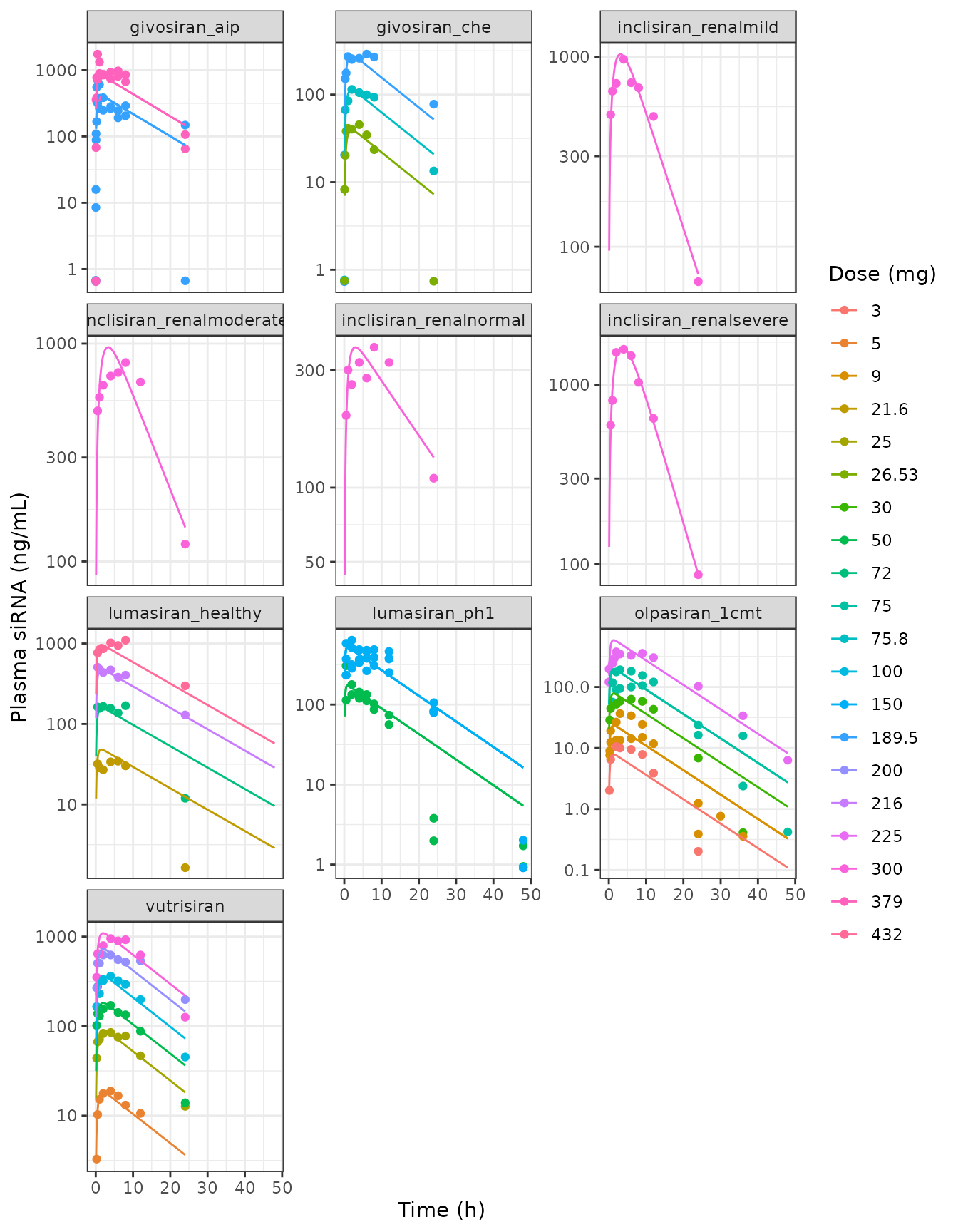
The fit of each model to its own data is summarised by the log10 ratio of prediction to observation:
fit1 <- obs1 |>
  filter(time > 0) |>
  group_by(model, id, dose) |>
  group_modify(\(x, key) {
    p <- sim_profile(key$model, key$dose, x$time)
    mutate(x, pred = p$Cc[match(x$time, p$time)])
  }) |>
  ungroup() |>
  mutate(lr = log10(pred / conc))
fit1_sum <- fit1 |>
  group_by(model) |>
  summarise(
    n = n(),
    `median log10(pred/obs)` = round(median(lr), 3),
    `median abs log10(pred/obs)` = round(median(abs(lr)), 3)
  )
knitr::kable(fit1_sum)| model | n | median log10(pred/obs) | median abs log10(pred/obs) |
|---|---|---|---|
| Sten_2023_givosiran_aip | 40 | 0.016 | 0.164 |
| Sten_2023_givosiran_che | 28 | -0.026 | 0.114 |
| Sten_2023_inclisiran_renalmild | 8 | 0.015 | 0.050 |
| Sten_2023_inclisiran_renalmoderate | 8 | 0.048 | 0.098 |
| Sten_2023_inclisiran_renalnormal | 8 | 0.010 | 0.081 |
| Sten_2023_inclisiran_renalsevere | 8 | -0.007 | 0.025 |
| Sten_2023_lumasiran_healthy | 28 | -0.011 | 0.057 |
| Sten_2023_lumasiran_ph1 | 48 | 0.046 | 0.104 |
| Sten_2023_olpasiran_1cmt | 62 | 0.060 | 0.175 |
| Sten_2023_vutrisiran | 53 | -0.016 | 0.063 |
stopifnot(
  # A mis-transcribed Ka, CL/F or V/F shifts a whole profile and moves the median
  # log ratio well beyond 0.1 (a 26% bias); every fit is centred on its own data.
  all(abs(fit1_sum$`median log10(pred/obs)`) < 0.1),
  all(fit1_sum$`median abs log10(pred/obs)` < 0.2)
)
NCA of the one-compartment models against the reported exposure
The ESM spreadsheet (sheet AUC_Cmax) also lists the
reported Cmax and AUC of the cohorts behind these profiles. The
one-compartment models are simulated at those doses and analysed with
PKNCA. AUC0-inf of a linear one-compartment model equals Dose/(CL/F)
exactly, which is also checked.
ref1 <- tribble(
  ~model, ~dose, ~aucinf.obs, ~cmax,
  "Sten_2023_vutrisiran", 5, 131, 19.6,
  "Sten_2023_vutrisiran", 25, 1020, 87.5,
  "Sten_2023_vutrisiran", 50, 2180, 178,
  "Sten_2023_vutrisiran", 100, 5200, 396,
  "Sten_2023_vutrisiran", 200, 12700, 727,
  "Sten_2023_vutrisiran", 300, 15500, 1090,
  "Sten_2023_lumasiran_healthy", 21.6, 294, 39.8,
  "Sten_2023_lumasiran_healthy", 72, 1900, 204,
  "Sten_2023_lumasiran_healthy", 216, 7210, 534,
  "Sten_2023_lumasiran_healthy", 432, 16800, 1180,
  "Sten_2023_givosiran_che", 26.53, 293, 52.1,
  "Sten_2023_givosiran_che", 75.8, 1180, 124,
  "Sten_2023_givosiran_che", 189.5, 4620, 356,
  "Sten_2023_inclisiran_renalnormal", 300, 7890, 421,
  "Sten_2023_inclisiran_renalmild", 300, 11600, 987,
  "Sten_2023_inclisiran_renalmoderate", 300, 10800, 897,
  "Sten_2023_inclisiran_renalsevere", 300, 18800, 1760
) |>
  mutate(treatment = paste(sub("Sten_2023_", "", model), dose, "mg"))

grid_nca <- c(seq(0, 12, by = 0.25), seq(13, 48, by = 1), seq(50, 240, by = 2))
conc1 <- ref1 |>
  rowwise() |>
  reframe(treatment, model, dose, sim_profile(model, dose, grid_nca)) |>
  mutate(id = 1L) |>
  filter(!is.na(Cc))
dose1 <- distinct(conc1, treatment, id, dose) |> mutate(time = 0)
o_conc <- PKNCAconc(conc1, Cc ~ time | treatment + id)
o_dose <- PKNCAdose(dose1, dose ~ time | treatment + id)
o_data <- PKNCAdata(o_conc, o_dose,
  intervals = data.frame(start = 0, end = Inf, cmax = TRUE, aucinf.obs = TRUE, half.life = TRUE)
)
nca1 <- as.data.frame(pk.nca(o_data))
tbl1 <- ncaComparisonTable(
  simulated = nca1,
  reference = select(ref1, treatment, aucinf.obs, cmax),
  by = "treatment",
  units = c(cmax = "ng/mL", aucinf.obs = "h*ng/mL"),
  tolerance_pct = 50
)
knitr::kable(tbl1, caption = attr(tbl1, "footnote"))| NCA parameter | treatment | Reference | Simulated | % diff |
|---|---|---|---|---|
| Cmax (ng/mL) | vutrisiran 5 mg | 19.6 | 18.2 | -7.2% |
| Cmax (ng/mL) | vutrisiran 25 mg | 87.5 | 90.9 | +3.9% |
| Cmax (ng/mL) | vutrisiran 50 mg | 178 | 182 | +2.2% |
| Cmax (ng/mL) | vutrisiran 100 mg | 396 | 364 | -8.1% |
| Cmax (ng/mL) | vutrisiran 200 mg | 727 | 728 | +0.1% |
| Cmax (ng/mL) | vutrisiran 300 mg | 1090 | 1090 | +0.1% |
| Cmax (ng/mL) | lumasiran_healthy 21.6 mg | 39.8 | 48.1 | +20.8% |
| Cmax (ng/mL) | lumasiran_healthy 72 mg | 204 | 160 | -21.5% |
| Cmax (ng/mL) | lumasiran_healthy 216 mg | 534 | 481 | -10.0% |
| Cmax (ng/mL) | lumasiran_healthy 432 mg | 1180 | 961 | -18.5% |
| Cmax (ng/mL) | givosiran_che 26.53 mg | 52.1 | 39.4 | -24.3% |
| Cmax (ng/mL) | givosiran_che 75.8 mg | 124 | 113 | -9.2% |
| Cmax (ng/mL) | givosiran_che 189.5 mg | 356 | 282 | -20.9% |
| Cmax (ng/mL) | inclisiran_renalnormal 300 mg | 421 | 372 | -11.7% |
| Cmax (ng/mL) | inclisiran_renalmild 300 mg | 987 | 1030 | +4.8% |
| Cmax (ng/mL) | inclisiran_renalmoderate 300 mg | 897 | 964 | +7.5% |
| Cmax (ng/mL) | inclisiran_renalsevere 300 mg | 1760 | 1620 | -7.9% |
| AUC0-∞ (obs) (h*ng/mL) | vutrisiran 5 mg | 131 | 281 | +114.3%* |
| AUC0-∞ (obs) (h*ng/mL) | vutrisiran 25 mg | 1020 | 1400 | +37.6% |
| AUC0-∞ (obs) (h*ng/mL) | vutrisiran 50 mg | 2180 | 2810 | +28.8% |
| AUC0-∞ (obs) (h*ng/mL) | vutrisiran 100 mg | 5200 | 5610 | +8.0% |
| AUC0-∞ (obs) (h*ng/mL) | vutrisiran 200 mg | 12700 | 11200 | -11.6% |
| AUC0-∞ (obs) (h*ng/mL) | vutrisiran 300 mg | 15500 | 16800 | +8.7% |
| AUC0-∞ (obs) (h*ng/mL) | lumasiran_healthy 21.6 mg | 294 | 860 | +192.5%* |
| AUC0-∞ (obs) (h*ng/mL) | lumasiran_healthy 72 mg | 1900 | 2870 | +50.9%* |
| AUC0-∞ (obs) (h*ng/mL) | lumasiran_healthy 216 mg | 7210 | 8600 | +19.3% |
| AUC0-∞ (obs) (h*ng/mL) | lumasiran_healthy 432 mg | 16800 | 17200 | +2.4% |
| AUC0-∞ (obs) (h*ng/mL) | givosiran_che 26.53 mg | 293 | 583 | +98.9%* |
| AUC0-∞ (obs) (h*ng/mL) | givosiran_che 75.8 mg | 1180 | 1660 | +41.1% |
| AUC0-∞ (obs) (h*ng/mL) | givosiran_che 189.5 mg | 4620 | 4160 | -9.9% |
| AUC0-∞ (obs) (h*ng/mL) | inclisiran_renalnormal 300 mg | 7890 | 8420 | +6.8% |
| AUC0-∞ (obs) (h*ng/mL) | inclisiran_renalmild 300 mg | 11600 | 11400 | -1.7% |
| AUC0-∞ (obs) (h*ng/mL) | inclisiran_renalmoderate 300 mg | 10800 | 13400 | +24.5% |
| AUC0-∞ (obs) (h*ng/mL) | inclisiran_renalsevere 300 mg | 18800 | 17600 | -6.2% |
# Closed form: AUC0-inf = 1000 * Dose / (CL/F) in h*ng/mL.
cl_of <- function(m) exp(unname(readModelDb(m)()$theta["lcl"]))
auc_check <- nca1 |>
  filter(PPTESTCD == "aucinf.obs") |>
  left_join(distinct(ref1, treatment, model, dose), by = "treatment") |>
  rowwise() |>
  mutate(closed = 1000 * dose / cl_of(model)) |>
  ungroup()
stopifnot(all(abs(auc_check$PPORRES / auc_check$closed - 1) < 0.01))
The one-compartment models, fitted to the first 24-48 h only, reproduce the reported Cmax of every cohort within about 25%. The inclisiran reported AUC0-inf rises with renal impairment (7890 to 18800 hng/mL) and the per-population CL/F of Table S4 falls in the same order (35.6 to 17.0 L/h). The rows flagged with a star (more than 50% difference) are the lowest doses of vutrisiran, lumasiran and givosiran. Within each of those cohorts the reported dose-normalised AUC rises with dose (vutrisiran 26 hng/mL per mg at 5 mg against 52-64 at 100-300 mg), which one linear model per population, fitted to all doses at once, cannot follow; the closed-form check above confirms the models themselves are transcribed exactly.
Three-compartment models (Table 3, Fig. 5, ESM Fig. S1)
# The observed sampling times are added so every observation has a prediction.
grid3 <- sort(unique(c(seq(0, 48, by = 0.5), seq(50, 2016, by = 4), tc$time)))
pred3 <- bind_rows(lapply(
  c("Sten_2023_galnacSirna_3cmt", "Sten_2023_olpasiran_3cmt"),
  function(m) {
    tc |>
      distinct(id, drug, dose) |>
      rowwise() |>
      reframe(id, drug, dose, sim_profile(m, dose, grid3)) |>
      mutate(fit = m)
  }
))
obs_mean <- tc |>
  group_by(drug, dose, time) |>
  summarise(conc = mean(conc), .groups = "drop")
pred3_mean <- pred3 |>
  distinct(fit, drug, dose, time, Cc) |>
  filter(time > 0)
ggplot(filter(obs_mean, time <= 168), aes(time, conc, colour = factor(dose))) +
  geom_point() +
  geom_line(
    data = filter(pred3_mean, fit == "Sten_2023_galnacSirna_3cmt", time <= 168),
    aes(time, Cc)
  ) +
  facet_wrap(~drug, scales = "free") +
  scale_y_log10() +
  labs(
    x = "Time (h)", y = "Plasma siRNA (ng/mL)", colour = "Dose (mg)",
    title = "Joint three-compartment fit (lines) and mean data (points)"
  ) +
  theme_bw()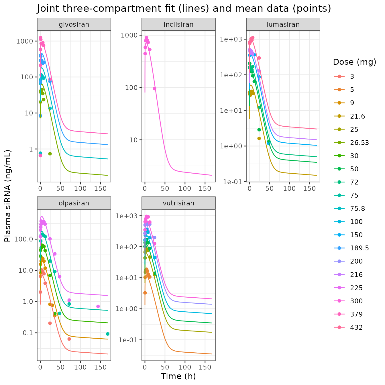
Replicates Figure 5 of Sten 2023 (first week); the olpasiran 12-week panel follows.
ggplot(filter(obs_mean, drug == "olpasiran"), aes(time / 24, conc, colour = factor(dose))) +
  geom_point() +
  geom_line(data = filter(pred3_mean, drug == "olpasiran"), aes(time / 24, Cc, linetype = fit)) +
  scale_y_log10() +
  labs(
    x = "Time (days)", y = "Plasma olpasiran (ng/mL)", colour = "Dose (mg)", linetype = NULL,
    title = "Olpasiran: joint fit and olpasiran-only fit"
  ) +
  theme_bw() +
  theme(legend.position = "bottom", legend.direction = "vertical")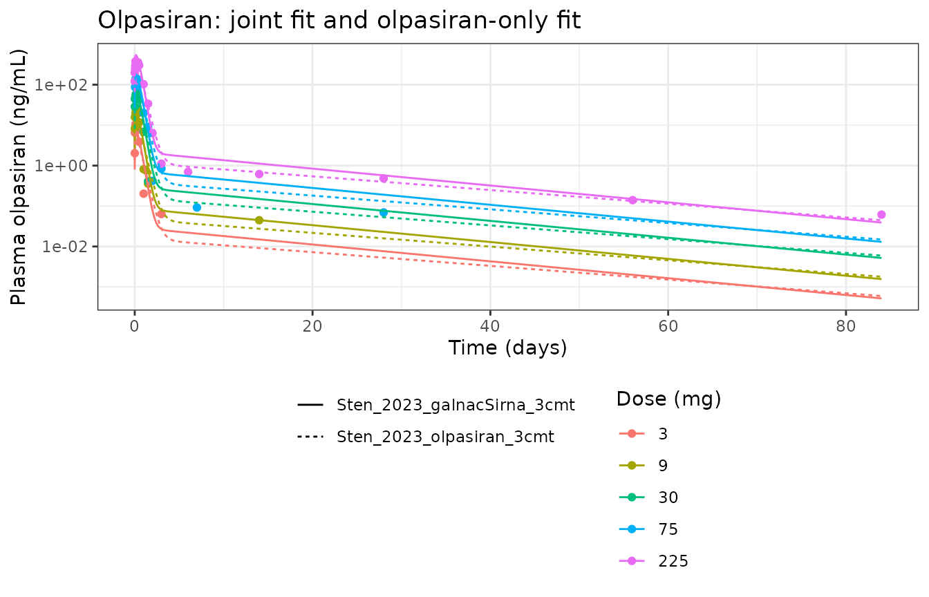
The olpasiran-only and joint fits agree for the first two days and both carry the long terminal phase (V2/F of 1470 and 1340 L) that Fig. 5 shows at 12 weeks.
fit3 <- pred3 |>
  inner_join(filter(tc, time > 0), by = c("id", "drug", "dose", "time")) |>
  mutate(lr = log10(Cc / conc))
fit3_sum <- bind_rows(
  fit3 |> filter(fit == "Sten_2023_galnacSirna_3cmt") |> group_by(fit, drug) |>
    summarise(n = n(), med = median(lr), mad = median(abs(lr)), .groups = "drop"),
  fit3 |> filter(fit == "Sten_2023_olpasiran_3cmt", drug == "olpasiran") |> group_by(fit, drug) |>
    summarise(n = n(), med = median(lr), mad = median(abs(lr)), .groups = "drop")
) |>
  mutate(across(c(med, mad), \(x) round(x, 3))) |>
  rename(`median log10(pred/obs)` = med, `median abs log10(pred/obs)` = mad)
knitr::kable(fit3_sum)| fit | drug | n | median log10(pred/obs) | median abs log10(pred/obs) |
|---|---|---|---|---|
| Sten_2023_galnacSirna_3cmt | givosiran | 68 | 0.187 | 0.206 |
| Sten_2023_galnacSirna_3cmt | inclisiran | 32 | -0.004 | 0.131 |
| Sten_2023_galnacSirna_3cmt | lumasiran | 76 | -0.006 | 0.108 |
| Sten_2023_galnacSirna_3cmt | olpasiran | 75 | 0.100 | 0.178 |
| Sten_2023_galnacSirna_3cmt | vutrisiran | 53 | -0.126 | 0.131 |
| Sten_2023_olpasiran_3cmt | olpasiran | 75 | -0.020 | 0.149 |
stopifnot(
  # The joint fit is one parameter set for five compounds, so per-compound bias up to
  # about 0.2 log10 (1.6-fold) is inside the twofold band Sten 2023 report around the
  # class-level regressions; a swapped V2/V3 or CL2/CL3 pair moves it far beyond this.
  all(abs(fit3_sum$`median log10(pred/obs)`) < 0.25),
  all(fit3_sum$`median abs log10(pred/obs)` < 0.25)
)
NCA of the joint model against the dose-exposure regressions (Table 2)
Table 2 reports class-level regressions in humans, AUC = 10^1.45 x Dose^1.05 and Cmax = 10^0.470 x Dose^0.989 (Dose in mg, AUC in h*ng/mL, Cmax in ng/mL), with a twofold band covering most of the data. The joint three-compartment model should fall inside that band.
doses_nca <- c(25, 100, 300)
grid_long <- sort(unique(c(seq(0, 24, by = 0.25), seq(25, 168, by = 1), seq(170, 4032, by = 8))))
conc3 <- bind_rows(lapply(doses_nca, function(d) {
  sim_profile("Sten_2023_galnacSirna_3cmt", d, grid_long) |>
    mutate(treatment = paste(d, "mg"), dose = d, id = 1L)
}))
d3 <- distinct(conc3, treatment, id, dose) |> mutate(time = 0)
nca3 <- pk.nca(PKNCAdata(
  PKNCAconc(conc3, Cc ~ time | treatment + id),
  PKNCAdose(d3, dose ~ time | treatment + id),
  intervals = data.frame(start = 0, end = Inf, cmax = TRUE, tmax = TRUE, aucinf.obs = TRUE)
))
ref3 <- data.frame(
  treatment = paste(doses_nca, "mg"),
  aucinf.obs = 10^1.45 * doses_nca^1.05,
  cmax = 10^0.470 * doses_nca^0.989
)
tbl3 <- ncaComparisonTable(
  simulated = as.data.frame(nca3),
  reference = ref3,
  by = "treatment",
  params = c("cmax", "aucinf.obs"),
  units = c(cmax = "ng/mL", aucinf.obs = "h*ng/mL"),
  tolerance_pct = 100
)
knitr::kable(tbl3, caption = attr(tbl3, "footnote"))| NCA parameter | treatment | Reference | Simulated | % diff |
|---|---|---|---|---|
| Cmax (ng/mL) | 25 mg | 71.2 | 59.7 | -16.2% |
| Cmax (ng/mL) | 100 mg | 281 | 239 | -14.9% |
| Cmax (ng/mL) | 300 mg | 832 | 717 | -13.8% |
| AUC0-∞ (obs) (h*ng/mL) | 25 mg | 828 | 1050 | +26.8% |
| AUC0-∞ (obs) (h*ng/mL) | 100 mg | 3550 | 4200 | +18.3% |
| AUC0-∞ (obs) (h*ng/mL) | 300 mg | 11200 | 12600 | +12.0% |
sim3 <- as.data.frame(nca3) |>
  filter(PPTESTCD %in% c("cmax", "aucinf.obs")) |>
  left_join(pivot_longer(ref3, -treatment, names_to = "PPTESTCD", values_to = "ref"),
    by = c("treatment", "PPTESTCD")
  )
stopifnot(all(sim3$PPORRES / sim3$ref > 0.5 & sim3$PPORRES / sim3$ref < 2))
The terminal half-life of the joint model follows from its smallest eigenvalue:
th <- function(m) {
  p <- exp(readModelDb(m)()$theta)
  k <- matrix(c(
    -(p[["lcl"]] + p[["lq"]] + p[["lq2"]]) / p[["lvc"]], p[["lq"]] / p[["lvp"]], p[["lq2"]] / p[["lvp2"]],
    p[["lq"]] / p[["lvc"]], -p[["lq"]] / p[["lvp"]], 0,
    p[["lq2"]] / p[["lvc"]], 0, -p[["lq2"]] / p[["lvp2"]]
  ), 3, byrow = TRUE)
  log(2) / min(abs(eigen(k)$values)) / 24
}
c(joint_days = th("Sten_2023_galnacSirna_3cmt"), olpasiran_only_days = th("Sten_2023_olpasiran_3cmt"))
#>          joint_days olpasiran_only_days
#>            14.45723            17.76669
Both fits give a terminal plasma half-life of several weeks, the redistribution-driven phase the abstract describes.
Corrected Ayyar 2021 mPBPK-PD model (ESM)
The ESM gives MATLAB scripts that regenerate Ayyar 2021 Figs. 2-5 with the corrected model and shows their output. The packaged models are simulated with the same doses, and the extremes the maintainers read off the ESM panels are checked below (deterministic model, so the comparison is exact up to the reading precision of the plots).
pbpk_run <- function(species, bw, mgkg, tend, dose_times = 0) {
  mod <- readModelDb(paste0("Sten_2023_fitusiran_mpbpk_", species))
  bind_rows(lapply(mgkg, function(d) {
    ev <- et(amt = d * bw, cmt = "depot", time = dose_times) |> et(seq(0, tend, by = 1))
    as.data.frame(rxSolve(mod, ev, atol = 1e-10, rtol = 1e-8, returnType = "data.frame")) |>
      mutate(dose_mgkg = d)
  }))
}
nadir <- function(sim) {
  sim |>
    group_by(dose_mgkg) |>
    summarise(
      mrna_min = min(mrna_liver), t_mrna = time[which.min(mrna_liver)],
      protein_min = min(protein), t_protein = time[which.min(protein)],
      risc_max = max(Crisc), t_risc = time[which.max(Crisc)],
      liver_max = max(Cliver)
    )
}
Mouse (Ayyar 2021 Fig. 2; 1, 2.5 and 5 mg/kg SC)
s_mouse <- pbpk_run("mouse", 0.028, c(1, 2.5, 5), 1000)
n_mouse <- nadir(s_mouse)
knitr::kable(n_mouse, digits = 2)| dose_mgkg | mrna_min | t_mrna | protein_min | t_protein | risc_max | t_risc | liver_max |
|---|---|---|---|---|---|---|---|
| 1.0 | 48.32 | 147 | 34.03 | 174 | 1.30 | 138 | 4427.46 |
| 2.5 | 29.54 | 145 | 16.36 | 174 | 3.22 | 140 | 11233.46 |
| 5.0 | 19.91 | 148 | 9.07 | 179 | 6.31 | 144 | 22811.37 |
s_mouse |>
  select(time, dose_mgkg, `Liver (ng/g)` = Cliver, `RISC-bound (ng/g)` = Crisc,
    `Liver mRNA (%)` = mrna_liver, `Plasma protein (%)` = protein) |>
  pivot_longer(-c(time, dose_mgkg)) |>
  ggplot(aes(time, value, colour = factor(dose_mgkg))) +
  geom_line() +
  facet_wrap(~name, scales = "free_y") +
  labs(x = "Time (h)", y = NULL, colour = "Dose (mg/kg)") +
  theme_bw()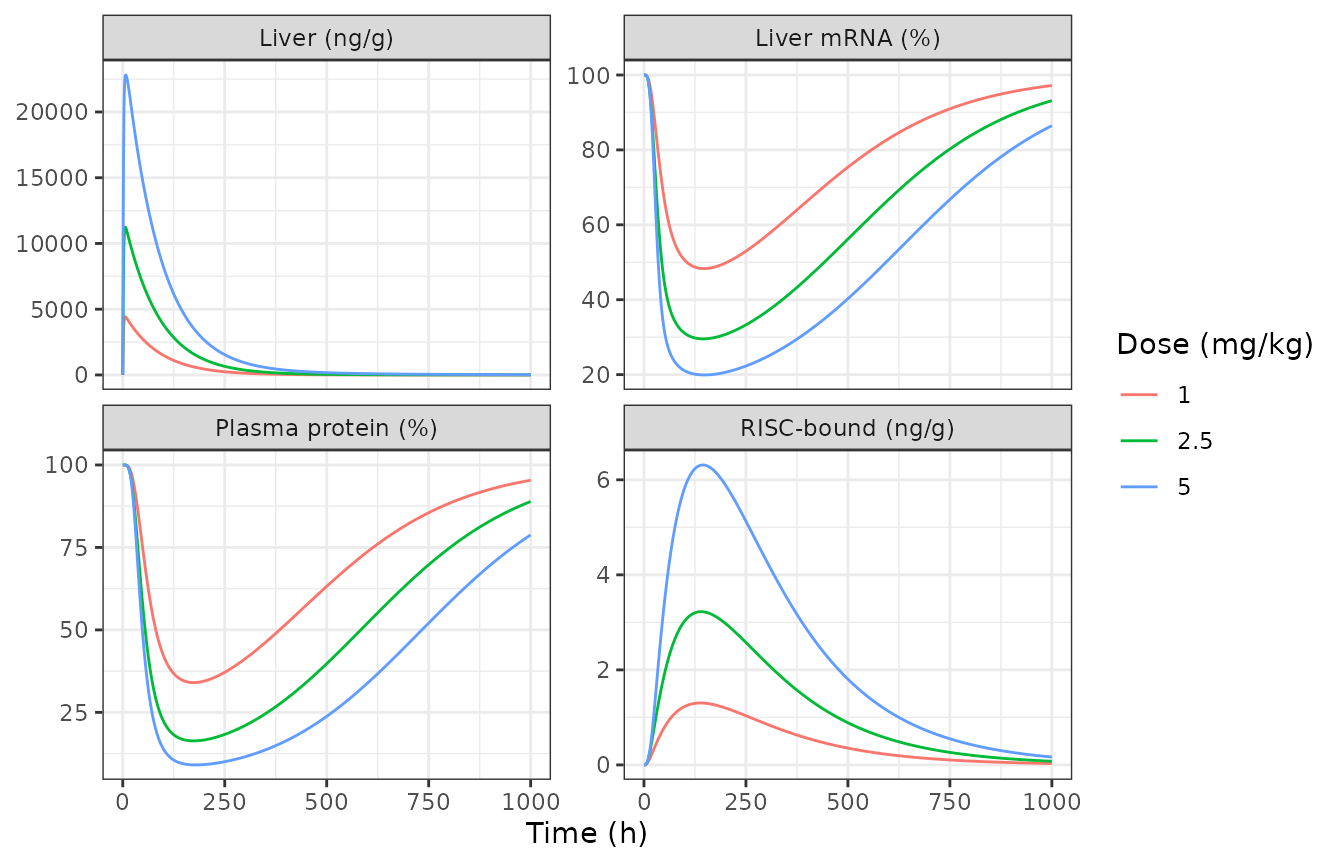
# Read from the ESM panels: mRNA nadir ~48 / ~29 / ~20 %, protein nadir ~34 / ~16 / ~9 %,
# RISC-bound peak ~3.2 ng/g near 140 h at 2.5 mg/kg.
stopifnot(
  all(abs(n_mouse$mrna_min / c(48, 29, 20) - 1) < 0.1),
  all(abs(n_mouse$protein_min / c(34, 16, 9) - 1) < 0.15),
  abs(n_mouse$risc_max[2] / 3.2 - 1) < 0.1
)
Rat (Ayyar 2021 Fig. 3; 1, 5 and 10 mg/kg SC)
s_rat <- pbpk_run("rat", 0.28, c(1, 5, 10), 700)
n_rat <- nadir(s_rat)
knitr::kable(n_rat, digits = 2)| dose_mgkg | mrna_min | t_mrna | protein_min | t_protein | risc_max | t_risc | liver_max |
|---|---|---|---|---|---|---|---|
| 1 | 49.55 | 127 | 35.65 | 155 | 1.24 | 118 | 7734.25 |
| 5 | 21.28 | 148 | 10.14 | 179 | 5.63 | 144 | 39837.11 |
| 10 | 15.58 | 185 | 6.29 | 214 | 9.85 | 183 | 80124.76 |
# Read from the ESM panels: RISC-bound peak ~1.2 ng/g (1 mg/kg) and ~5.6 ng/g (5 mg/kg);
# 10 mg/kg liver concentration peaks just under 1e5 ng/g and is ~1e4 ng/g at 300 h.
stopifnot(
  all(abs(n_rat$risc_max[1:2] / c(1.2, 5.6) - 1) < 0.1),
  n_rat$liver_max[3] > 5e4 && n_rat$liver_max[3] < 1e5,
  abs(log10(s_rat$Cliver[s_rat$dose_mgkg == 10 & s_rat$time == 300] / 1e4)) < 0.15
)
Cynomolgus monkey (Ayyar 2021 Fig. 4; 1, 3, 10 and 30 mg/kg SC)
s_monkey <- pbpk_run("monkey", 6.2, c(1, 3, 10, 30), 1500)
n_monkey <- nadir(s_monkey)
knitr::kable(n_monkey, digits = 2)| dose_mgkg | mrna_min | t_mrna | protein_min | t_protein | risc_max | t_risc | liver_max |
|---|---|---|---|---|---|---|---|
| 1 | 48.72 | 157 | 47.20 | 305 | 2.83 | 149 | 9968.41 |
| 3 | 27.88 | 179 | 24.17 | 363 | 7.86 | 174 | 30658.59 |
| 10 | 16.08 | 267 | 10.49 | 475 | 20.48 | 265 | 103523.98 |
| 30 | 12.43 | 579 | 5.26 | 689 | 34.71 | 577 | 312171.30 |
ggplot(s_monkey, aes(time, protein, colour = factor(dose_mgkg))) +
  geom_line() +
  labs(x = "Time (h)", y = "Plasma antithrombin (%)", colour = "Dose (mg/kg)") +
  theme_bw()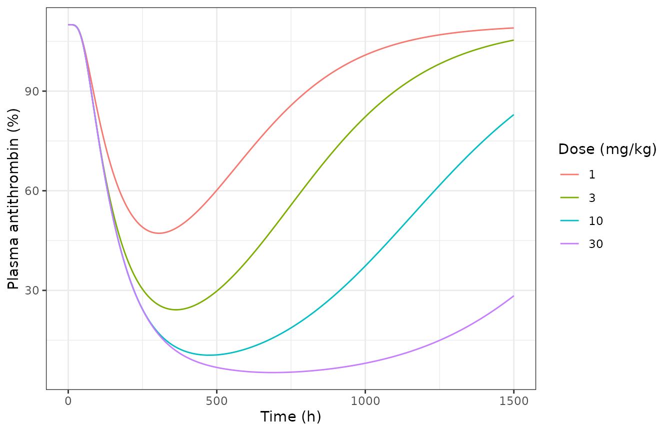
Human (Ayyar 2021 Fig. 5)
Three monthly doses of 80 mg or 0.225 mg/kg, three weekly doses of 0.015 mg/kg, a single dose of 0.03 mg/kg (Fig. 5B) and three monthly doses of 1.8 or 0.45 mg/kg (Fig. 5C), in a 71 kg adult.
q4w <- c(0, 28, 56) * 24
s_h <- bind_rows(
  pbpk_run("human", 71, c(80 / 71, 0.225, 1.8, 0.45), 6000, q4w) |> mutate(regimen = "Q4W x3"),
  pbpk_run("human", 71, 0.015, 6000, c(0, 7, 14) * 24) |> mutate(regimen = "QW x3"),
  pbpk_run("human", 71, 0.03, 6000) |> mutate(regimen = "single")
) |>
  mutate(label = paste(signif(dose_mgkg, 3), "mg/kg", regimen))
n_h <- s_h |>
  group_by(label) |>
  summarise(protein_min = min(protein), t_protein = time[which.min(protein)])
knitr::kable(n_h, digits = 2)| label | protein_min | t_protein |
|---|---|---|
| 0.015 mg/kg QW x3 | 87.11 | 716 |
| 0.03 mg/kg single | 90.68 | 481 |
| 0.225 mg/kg Q4W x3 | 35.20 | 1720 |
| 0.45 mg/kg Q4W x3 | 20.60 | 1719 |
| 1.13 mg/kg Q4W x3 | 9.36 | 1718 |
| 1.8 mg/kg Q4W x3 | 6.43 | 1722 |
ggplot(s_h, aes(time, protein, colour = label)) +
  geom_line() +
  labs(x = "Time (h)", y = "Plasma antithrombin (%)", colour = NULL) +
  theme_bw()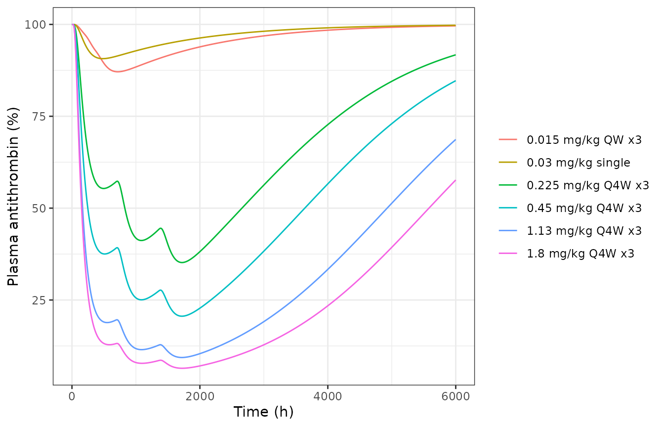
nh <- setNames(n_h$protein_min, n_h$label)
# Read from the ESM panels: nadirs ~9.5 (80 mg), ~35 (0.225 mg/kg), ~6.5 (1.8 mg/kg),
# ~20.5 (0.45 mg/kg), ~87 (0.015 mg/kg QW) and ~90.5 % (0.03 mg/kg single).
stopifnot(
  abs(nh[["1.13 mg/kg Q4W x3"]] / 9.5 - 1) < 0.15,
  abs(nh[["0.225 mg/kg Q4W x3"]] / 35 - 1) < 0.1,
  abs(nh[["1.8 mg/kg Q4W x3"]] / 6.5 - 1) < 0.15,
  abs(nh[["0.45 mg/kg Q4W x3"]] / 20.5 - 1) < 0.1,
  abs(nh[["0.015 mg/kg QW x3"]] - 87) < 3,
  abs(nh[["0.03 mg/kg single"]] - 90.5) < 3
)
Olpasiran plasma profile with the human mPBPK model (Fig. 6)
Sten 2023 Fig. 6 compares the human parameter set with the olpasiran data: it captures the first days but falls well below the observed concentrations beyond 168 h. The same comparison, with the mPBPK model and the joint three-compartment model side by side:
olp_doses <- c(3, 9, 30, 75, 225)
grid6 <- sort(unique(c(seq(0, 48, by = 0.5), seq(50, 2016, by = 4))))
p6 <- bind_rows(lapply(olp_doses, function(d) {
  mod <- readModelDb("Sten_2023_fitusiran_mpbpk_human")
  out <- as.data.frame(rxSolve(mod, et(amt = d, cmt = "depot") |> et(grid6),
    atol = 1e-10, rtol = 1e-8, returnType = "data.frame"
  ))
  data.frame(dose = d, time = out$time, Cc = out$Cc, model = "mPBPK (human)")
}))
p6 <- bind_rows(
  p6,
  pred3_mean |>
    filter(fit == "Sten_2023_galnacSirna_3cmt", drug == "olpasiran") |>
    transmute(dose, time, Cc, model = "joint three-compartment")
)
ggplot(filter(obs_mean, drug == "olpasiran", time <= 336), aes(time, conc, colour = factor(dose))) +
  geom_point() +
  geom_line(data = filter(p6, time > 0, time <= 336), aes(time, Cc, linetype = model)) +
  scale_y_log10(limits = c(1e-3, 1e3)) +
  labs(x = "Time (h)", y = "Plasma olpasiran (ng/mL)", colour = "Dose (mg)", linetype = NULL) +
  theme_bw()
#> Warning: Removed 51 rows containing missing values or values outside the scale range
#> (`geom_line()`).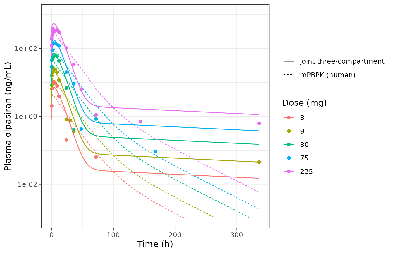
Baseline steady state
Without a dose every receptor, mRNA and protein state must stay at its baseline (free ASGPR = Rtot because ksyn = Rtot x kdeg, correction 4 of the ESM).
ss <- bind_rows(lapply(c("mouse", "rat", "monkey", "human"), function(sp) {
  mod <- readModelDb(paste0("Sten_2023_fitusiran_mpbpk_", sp))
  th <- mod()$theta
  out <- as.data.frame(rxSolve(mod, et(seq(0, 2000, by = 500)), returnType = "data.frame"))
  data.frame(
    species = sp,
    target_dev = max(abs(out$target / th[["rtot"]] - 1)),
    mrna_dev = max(abs(out$mrna_liver / th[["mrna0"]] - 1)),
    protein_dev = max(abs(out$protein / th[["protein0"]] - 1))
  )
}))
knitr::kable(ss, digits = 12)| species | target_dev | mrna_dev | protein_dev |
|---|---|---|---|
| mouse | 0 | 0 | 0 |
| rat | 0 | 0 | 0 |
| monkey | 0 | 0 | 0 |
| human | 0 | 0 | 0 |
Assumptions and deviations
-
Residual error. Sten 2023 does not report the
residual-error model of the WinNonlin naive-pooled fits, so the
compartmental files carry
propSd = fixed(0). They are typical-value (group-mean) models and should not be used to simulate between-subject variability. -
Naive pooling. The population sizes in each
populationelement are the sums of the per-arm group sizes the ESM spreadsheet lists for the cohorts behind the profiles; the fits themselves used only the group means. For the joint three-compartment model the subject count is left unset. - One-compartment files are per population, not a covariate model. Sten 2023 fitted each compound / population separately (Table S4); the files reproduce that structure instead of combining, for example, the four inclisiran renal-function fits into one model with renal indicators.
- mPBPK-PD units. The ESM code doses the depot in ng; the packaged models take the dose in mg and convert (x 1e6) where the depot feeds plasma. The other states keep the units of the ESM code (plasma, remainder, kidney vascular and liver vascular in ng/mL, kidney tissue in ng/g, kidney bound pool in ng, liver bound pool in nmol, receptor and intracellular states in nM, mRNA and protein in percent of baseline), so they are concentrations rather than amounts.
-
mPBPK-PD body weight. The allometric scaling and
mg/kg dosing use one typical weight per species (
bw, a fixed parameter), as in the ESM scripts. Simulating another animal size means changingbw(and the physiological volumes and flows, which the ESM gives only for these four weights). - SC50 unit. The mouse and rat branches of the ESM code print the SC50 unit as “ng/M”; it is compared with the RISC-bound siRNA concentration in nM and is treated as nM.
- Rat PD parameters. The ESM marks the rat kdeg_mRNA, kdeg_protein, Smax, SC50 and gamma as not available in Ayyar 2021 and carries the mouse values; the packaged rat file does the same.
- Monkey baseline protein. The monkey parameter set uses protein0 = 110% (assigned by Sten 2023 from Ayyar 2021 Fig. 4); the steady-state check above uses this baseline.
- Drug name of the mPBPK-PD files. The model is a generic GalNAc-siRNA framework, but its PD layer (antithrombin mRNA and protein) and calibration come from fitusiran, so the files are named for fitusiran. Sten 2023 applies the human parameter set to olpasiran plasma data only (Fig. 6), as above.
- Table 2 regressions are statistical summaries and are not packaged; they are used only as an external check on the joint three-compartment model.
- Figure read-offs. The PBPK check values are read by the maintainers from the panels the ESM prints for its own MATLAB runs; tolerances (10-15%, or 0.15 log10 for the log-scale plasma values) reflect the reading precision of those plots.