Finerenone UACR and eGFR dose-exposure-response (Goulooze 2022)
Source:vignettes/articles/Goulooze_2022_finerenone_uacr_egfr.Rmd
Goulooze_2022_finerenone_uacr_egfr.RmdModel and source
This paper contributed two model files, matching the two sequential NONMEM runs the authors performed.
uacrMod <- readModelDb("Goulooze_2022_finerenone_uacr")
egfrMod <- readModelDb("Goulooze_2022_finerenone_egfr")- Citation: Goulooze SC, Heerspink HJL, van Noort M, Snelder N, Brinker M, Lippert J, Eissing T. Dose-Exposure-Response Analysis of the Nonsteroidal Mineralocorticoid Receptor Antagonist Finerenone on UACR and eGFR: An Analysis from FIDELIO-DKD. Clin Pharmacokinet. 2022;61(7):1013-1025. doi:10.1007/s40262-022-01124-3. Parameter values are the final estimates in Table S1 of the Electronic Supplementary Material; the model equations are the final UACR NONMEM control stream in the same supplement. The exposure metric AUCtau,md is computed from the upstream FIDELIO-DKD population PK analysis (van den Berg P et al., Clin Pharmacokinet. 2022;61(3):439-450; doi:10.1007/s40262-021-01082-2); see modellib(‘vandenBerg_2021_finerenone’).
- UACR model: Population PKPD disease-progression model for the urine albumin-to-creatinine ratio (UACR) response to finerenone in patients with chronic kidney disease and type 2 diabetes (FIDELIO-DKD Phase III). UACR is integrated as a state whose fractional progression rate is corrected by the model-predicted UACR and by UACR over baseline; the finerenone effect is a power function of steady-state daily AUC acting through an effect compartment, and concomitant SGLT2 inhibitor use gives a direct proportional shift. Finerenone PK is upstream (van den Berg 2022) and reduced here to AUCss = DOSE / CL with typical apparent clearance 29.9 L/h.
- eGFR model: Population PKPD disease-progression model for the estimated glomerular filtration rate (eGFR) response to finerenone in patients with chronic kidney disease and type 2 diabetes (FIDELIO-DKD Phase III). eGFR declines at a constant chronic slope that is flattened by an exponential stabilisation function as eGFR approaches 16.1 mL/min/1.73 m^2, and the chronic slope is driven by the model-predicted UACR time course from the companion UACR model rather than by baseline UACR. Finerenone acts twice: an acute fully reversible eGFR decline through a power function of steady-state daily AUC acting via its own effect compartment, and, via its UACR reduction, a sustained flattening of the chronic slope. Finerenone PK is upstream (van den Berg 2022) and reduced here to AUCss = DOSE / CL with typical apparent clearance 29.9 L/h.
- Article: https://doi.org/10.1007/s40262-022-01124-3
- Supplement (Electronic Supplementary Material, Tables S1 / S2 and both final NONMEM control streams): https://doi.org/10.1007/s40262-022-01124-3
- Upstream population PK providing the exposure metric: https://doi.org/10.1007/s40262-021-01082-2
(
modellib("vandenBerg_2021_finerenone"))
FIDELIO-DKD randomised 5,734 patients with chronic kidney disease (CKD) and type 2 diabetes to finerenone 10 or 20 mg once daily or placebo, on top of standard of care including a maximally tolerated labelled dose of a renin-angiotensin system inhibitor. This secondary analysis quantified the dose-exposure-response relationship for two surrogate endpoints of CKD progression, the urine albumin-to-creatinine ratio (UACR) and the estimated glomerular filtration rate (eGFR), and asked whether concomitant SGLT2 inhibitor (SGLT2i) use modifies the finerenone effect.
The authors fitted the two endpoints sequentially:
- A UACR disease-progression model, on placebo data first and then on the full dataset with the finerenone effect added.
- An eGFR disease-progression model, which embeds the UACR sub-model and uses the model-predicted UACR time course (not baseline UACR) as the driver of the chronic eGFR slope. In the source, that sub-model’s parameters enter the eGFR run as data columns holding the individual post-hoc estimates from step 1.
Because the eGFR run holds those UACR parameters fixed, the packaged
eGFR model reproduces them as fixed() typical values from
ESM Table S1 so that the file is self-contained. Fitting the eGFR model
to real data would instead supply individual post-hoc UACR parameters,
exactly as the authors did.
The paper’s central finding is that no UACR-independent finerenone effect on the chronic eGFR slope was identifiable: once the model-predicted UACR drives the slope, the drug’s long-term eGFR benefit follows entirely from its early UACR reduction.
Population
The analysis included 5,674 patients (the FIDELIO-DKD full analysis set) with 37,296 UACR and 78,132 eGFR observations. Median age was 66-67 years, median body weight 84.6-87.6 kg, and 29.4% were female. Median baseline eGFR ranged from 42.1 to 51.3 mL/min/1.73 m^2 and median baseline UACR from 661 to 887 mg/g across the four treatment / SGLT2i groups of Table 1. 528 patients used an SGLT2 inhibitor at some point during the treatment period. Race was 63.2% White, 4.6% Black or African American, 7.3% Japanese, 10.3% Chinese and 14.4% other (pooled across the four groups of Table 1).
The same information is available programmatically from either
model’s population metadata.
str(readModelDb("Goulooze_2022_finerenone_egfr")()$population, max.level = 1)
#> List of 11
#>  $ species       : chr "human"
#>  $ n_subjects    : int 5674
#>  $ n_studies     : int 1
#>  $ age_range     : chr "adults; median 66-67 years (IQR approximately 57-72) across treatment groups"
#>  $ weight_range  : chr "median 84.6-87.6 kg (IQR approximately 72.6-99.4) across treatment groups"
#>  $ sex_female_pct: num 29.4
#>  $ race_ethnicity: Named num [1:5] 63.2 4.6 7.3 10.3 14.4
#>   ..- attr(*, "names")= chr [1:5] "White" "Black" "Japanese" "Chinese" ...
#>  $ disease_state : chr "Chronic kidney disease with type 2 diabetes mellitus; baseline eGFR median 42.1-51.3 mL/min/1.73 m^2 and baseli"| __truncated__
#>  $ dose_range    : chr "Oral finerenone 10 mg or 20 mg once daily (starting dose 10 mg if screening eGFR 25 to < 60 mL/min/1.73 m^2, 20"| __truncated__
#>  $ regions       : chr "Multi-regional Phase III (FIDELIO-DKD, NCT02540993)"
#>  $ notes         : chr "78,132 eGFR observations from 5,674 patients (full analysis set). 528 patients used an SGLT2 inhibitor at some "| __truncated__
Source trace
Per-parameter origins are recorded as in-file comments next to each
ini() entry. All values are the final
estimates in ESM Tables S1 and S2; the $THETA blocks of the
supplement’s control streams hold initial estimates (for
example eGFR TH1 initial 3.79 vs final 3.77, TH2 initial 3.1 vs final
3.01) and were used only for the equation forms.
UACR model (Goulooze_2022_finerenone_uacr)
| Equation / parameter | Value | Source location |
|---|---|---|
lrbase (typical baseline UACR) |
866 mg/g | ESM Table S1, theta_pop,BSLUACR |
prog (progression rate) |
0.137 /year | ESM Table S1, theta_pop,PROG |
cslope1 |
7.20e-5 g/mg/year | ESM Table S1, theta_pop,CSLOPE1 |
cslope2 |
0.182 /year | ESM Table S1, theta_pop,CSLOPE2 |
eslope (drug effect slope) |
-1.42 | ESM Table S1, theta_pop,ESLOPE |
epow |
0.613 | ESM Table S1, theta_pop,EPOW |
eslope2 |
-1.66e-4 g/mg | ESM Table S1, theta_pop,ESLOPE2 |
lke0 |
1.36e-4 /h | ESM Table S1, theta_pop,KE0,UACR |
e_uacr_rbase |
0.877 | ESM Table S1, theta_UACR0,BSLUACR |
e_crcl_rbase |
-0.124 | ESM Table S1, theta_EGFREPI0,BSLUACR |
e_hepimp_mod_rbase |
0.0943 | ESM Table S1, theta_CHILDPUGH,BSLUACR |
e_crcl_prog |
-0.00257 | ESM Table S1, theta_EGFREPI0,PROG |
e_race_asian_prog |
0.0634 /year | ESM Table S1, theta_ASIAN,PROG |
e_age_eslope |
0.864 | ESM Table S1, theta_AGE,ESLOPE |
e_race_japanese_eslope |
-0.261 | ESM Table S1, theta_JAPAN,ESLOPE |
e_conmed_sglt2i_uacr |
-0.212 | ESM Table S1, theta_SGLT2i,UACR |
boxcox_prog, boxcox_eslope
|
-0.545, -0.955 | ESM Table S1, BOXCOX PROG / ESLOPE |
| omega block (BSLUACR, PROG, ESLOPE) | see ini()
|
ESM Table S1, omega^2 and covariance rows |
expSd |
sqrt(0.141) | ESM Table S1, sigma^2 (additive on log-scale) |
d/dt(uacr), d/dt(effect), observation |
n/a | ESM, UACR control stream $DES /
$ERROR
|
lcl (exposure metric denominator) |
29.9 L/h | van den Berg 2022 Table 2 (upstream) |
eGFR model (Goulooze_2022_finerenone_egfr)
| Equation / parameter | Value | Source location |
|---|---|---|
lrbase_egfr |
ln = 3.77 | ESM Table S2, theta_pop,BSLEGFR |
pdecline (PMAX) |
3.01 mL/min/1.73 m^2/year | ESM Table S2, theta_pop,PMAX |
lpint (fixed) |
ln = 2.78 | ESM Table S2, theta_pop,PINT (fixed to the placebo model) |
pslope (fixed) |
-0.300 | ESM Table S2, theta_pop,PSLOPE (fixed to the placebo model) |
lke0 |
0.00230 /h | ESM Table S2, theta_pop,KE0,eGFR |
ldslope (DSLOPE) |
0.0475 | ESM Table S2, theta_pop,DSLOPE |
dpow (DPOW) |
0.555 | ESM Table S2, theta_pop,DPOW |
e_uacr_pdecline |
8.59e-4 | ESM Table S2, theta_UACR,PMAX |
e_crcl_uacr_pdecline |
-0.560 | ESM Table S2, theta_EGFREPI0,INTER |
e_crcl_rbase_egfr |
0.882 | ESM Table S2, theta_EGFREPI0,BSLEGFR |
e_crcl_pdecline |
0.387 | ESM Table S2, theta_EGFREPI0,PMAX |
e_race_black_pdecline |
1.24 | ESM Table S2, theta_BAA,PMAX |
e_hepimp_mod_pdecline |
1.18 | ESM Table S2, theta_CHILDPUGH,PMAX |
e_pot_dslope |
-1.38 | ESM Table S2, theta_K0,DSLOPE |
e_conmed_sglt2i_acute |
-0.0558 | ESM Table S2, theta_SGLT2i,acute,eGFR |
e_conmed_sglt2i_pdecline |
-0.457 | ESM Table S2, theta_SGLT2i,PMAX |
e_uacr_iiv_pdecline |
0.306 | ESM Table S2, theta_UACR0,IIV,PMAX |
boxcox_rbase_egfr, boxcox_pdecline
|
7.63, 0.145 | ESM Table S2, BOXCOX BSL / PROG |
omega block, etapdecline, etalpint
|
see ini()
|
ESM Table S2, omega^2 and covariance rows |
propSd, addSd
|
sqrt(0.0101), sqrt(2.01) | ESM Table S2, sigma^2 PROP / ADD |
embedded UACR sub-model (*_uacr names) |
see UACR table above | ESM Table S1 (held fixed in the eGFR run) |
d/dt(egfr), d/dt(effect1),
d/dt(uacr), d/dt(effect2), observation |
n/a | ESM, eGFR control stream $DES /
$ERROR
|
Units
Both models run on a time base of hours
(units$time = "h"), because the effect-compartment
equilibration rate constants are reported per hour. Annual rates are
converted inline. The two source control streams use
different year lengths and both are reproduced as
published: 365 days per year in the UACR model, 365.25 in the eGFR
model.
| Term | Units | Check |
|---|---|---|
uacr state |
mg/g | initial condition rbase in mg/g |
progRate * uacr |
mg/g/h | (1/year -> 1/h) x mg/g |
cslope1Hr * uacrDrug * uacr |
mg/g/h | (g/mg/year -> g/mg/h) x mg/g x mg/g |
cslope2Hr * log(uacrDrug/rbase) * uacr |
mg/g/h | (1/year -> 1/h) x unitless x mg/g |
effect state |
mg*h/L | equilibrates toward aucSs = mg / (L/h) |
aucSs = podo(depot)/cl |
mg*h/L | mg / (L/h) |
egfr state |
mL/min/1.73 m^2 | initial condition rbase_egfr
|
pdeclineHr |
mL/min/1.73 m^2 per h | (per year -> per h) |
(uacrDriver - 850) * e_uacr_pdecline |
unitless | mg/g x (per mg/g) |
pa20 * exp((egfr*(1-acuteEff) - 20) * pslope) |
mL/min/1.73 m^2 per h |
pslope in 1.73 m^2 min/mL makes the exponent
unitless |
acuteEff = effect1^dpow * dslope |
unitless | fractional reduction of eGFR at the observation |
Two consequences of the effect-compartment structure are worth naming, because they are what make the paper’s story work:
- Both finerenone effects (
acuteEffon eGFR,uacrEffon UACR) are applied at the observation, not inside the eGFR / UACR differential equations. That is what makes the acute eGFR decline fully reversible on discontinuation. - The chronic eGFR slope is driven by
uacrDriver, the drug- and SGLT2i-adjusted UACR, so a drug effect on UACR propagates into the eGFR slope without any separate eGFR drug-effect parameter.
Simulation setup
The published simulations in Figures 3 and 6 and Tables 3 and 4 are
typical-subject simulations at a constant dose, without
inter-individual or residual variability and without dose titration
(paper Sect. 2.3). Random effects are zeroed with
rxode2::zeroRe().
The exposure metric is the steady-state daily AUC, computed
algebraically as AUCtau,md = DOSE / CL with the upstream
typical apparent clearance of 29.9 L/h. podo(depot) reads
the most recent dose amount, so a single dose record at time 0
establishes a constant exposure, and an explicit amt = 0
record models discontinuation.
uacrTyp <- rxode2::zeroRe(rxode2::rxode2(uacrMod))
#> ℹ parameter labels from comments will be replaced by 'label()'
egfrTyp <- rxode2::zeroRe(rxode2::rxode2(egfrMod))
#> ℹ parameter labels from comments will be replaced by 'label()'

# Reference FIDELIO-DKD subject, Goulooze 2022 Table 3 footnote:
# UACR0 = 852 mg/g, EGFREPI0 = 43.0 mL/min/1.73 m^2, age = 66 years,
# K0 = 4.4 mmol/L, race not Asian nor Black or African American, not
# likely or certain Child-Pugh B.
refSubject <- list(
  UACR = 852, CRCL = 43, AGE = 66, POT = 4.4,
  HEPIMP_MOD = 0, RACE_ASIAN = 0, RACE_JAPANESE = 0, RACE_BLACK = 0,
  CONMED_SGLT2I_BASE = 0
)

obsTimes <- seq(0, 4 * 365 * 24, by = 24)   # 4 years, daily

# Build an event table: one dose record at time 0 (omitted for placebo), plus
# an optional amt = 0 record to model discontinuation.
makeEvents <- function(dose, stopTime = NA_real_) {
  ev <- rxode2::et(obsTimes)
  if (dose > 0) {
    ev <- rxode2::et(ev, amt = dose, time = 0, cmt = "depot")
  }
  if (!is.na(stopTime)) {
    ev <- rxode2::et(ev, amt = 0, time = stopTime, cmt = "depot")
  }
  ev
}

simTypical <- function(mod, dose, sglt2i, overrides = list(), stopTime = NA_real_) {
  pars <- utils::modifyList(refSubject, overrides)
  pars$CONMED_SGLT2I <- sglt2i
  as.data.frame(rxode2::rxSolve(
    mod,
    params     = unlist(pars),
    events     = makeEvents(dose, stopTime),
    returnType = "data.frame"
  ))
}
Replicate published figures
Figure 3A - UACR over baseline by finerenone dose
# Replicates Figure 3A of Goulooze 2022: simulated UACR over baseline for a
# typical patient not using an SGLT2 inhibitor, at 0 / 10 / 20 mg once daily.
fig3a <- bind_rows(lapply(c(0, 10, 20), function(d) {
  simTypical(uacrTyp, d, 0) |>
    transmute(
      years = time / (365 * 24),
      ratio = uacrObs / uacrObs[1],
      dose  = factor(d, levels = c(0, 10, 20),
                     labels = c("Placebo", "Finerenone 10 mg OD", "Finerenone 20 mg OD"))
    )
}))
#> ℹ omega/sigma items treated as zero: 'etalrbase', 'etaprog', 'etaeslope'
#> ℹ omega/sigma items treated as zero: 'etalrbase', 'etaprog', 'etaeslope'
#> ℹ omega/sigma items treated as zero: 'etalrbase', 'etaprog', 'etaeslope'

ggplot(fig3a, aes(years, ratio, colour = dose)) +
  geom_line(linewidth = 0.8) +
  scale_x_continuous(breaks = 0:4) +
  labs(x = "Time (years)", y = "UACR over baseline", colour = NULL,
       title = "Figure 3A - UACR dose-response in a typical patient",
       caption = "Replicates Figure 3A of Goulooze 2022.") +
  theme_bw() +
  theme(legend.position = "bottom")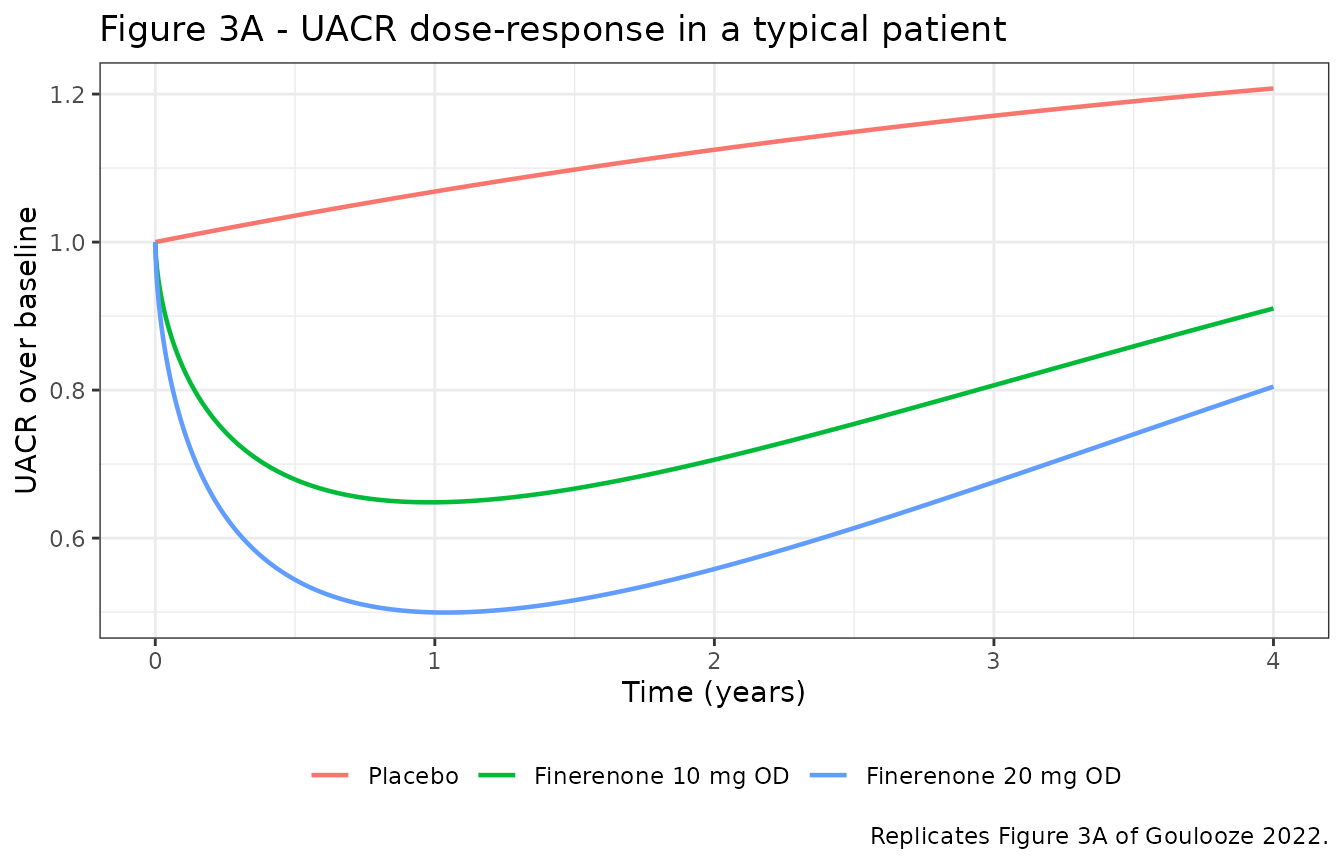
The 20 mg curve sits below the 10 mg curve but by less than a doubling of the effect, reproducing the paper’s observation that the UACR effect is already saturating between the two marketed doses.
Figure 3B - eGFR by finerenone dose
# Replicates Figure 3B of Goulooze 2022: simulated eGFR for a typical patient
# not using an SGLT2 inhibitor, at 0 / 10 / 20 mg once daily.
fig3b <- bind_rows(lapply(c(0, 10, 20), function(d) {
  simTypical(egfrTyp, d, 0) |>
    transmute(
      years = time / (365 * 24),
      egfr  = egfrObs,
      dose  = factor(d, levels = c(0, 10, 20),
                     labels = c("Placebo", "Finerenone 10 mg OD", "Finerenone 20 mg OD"))
    )
}))
#> ℹ omega/sigma items treated as zero: 'etalrbase_egfr', 'etaldslope', 'etapdecline', 'etalpint'
#> ℹ omega/sigma items treated as zero: 'etalrbase_egfr', 'etaldslope', 'etapdecline', 'etalpint'
#> ℹ omega/sigma items treated as zero: 'etalrbase_egfr', 'etaldslope', 'etapdecline', 'etalpint'

ggplot(fig3b, aes(years, egfr, colour = dose)) +
  geom_line(linewidth = 0.8) +
  scale_x_continuous(breaks = 0:4) +
  labs(x = "Time (years)", y = expression(eGFR~(mL/min/1.73~m^2)), colour = NULL,
       title = "Figure 3B - eGFR dose-response in a typical patient",
       caption = "Replicates Figure 3B of Goulooze 2022.") +
  theme_bw() +
  theme(legend.position = "bottom")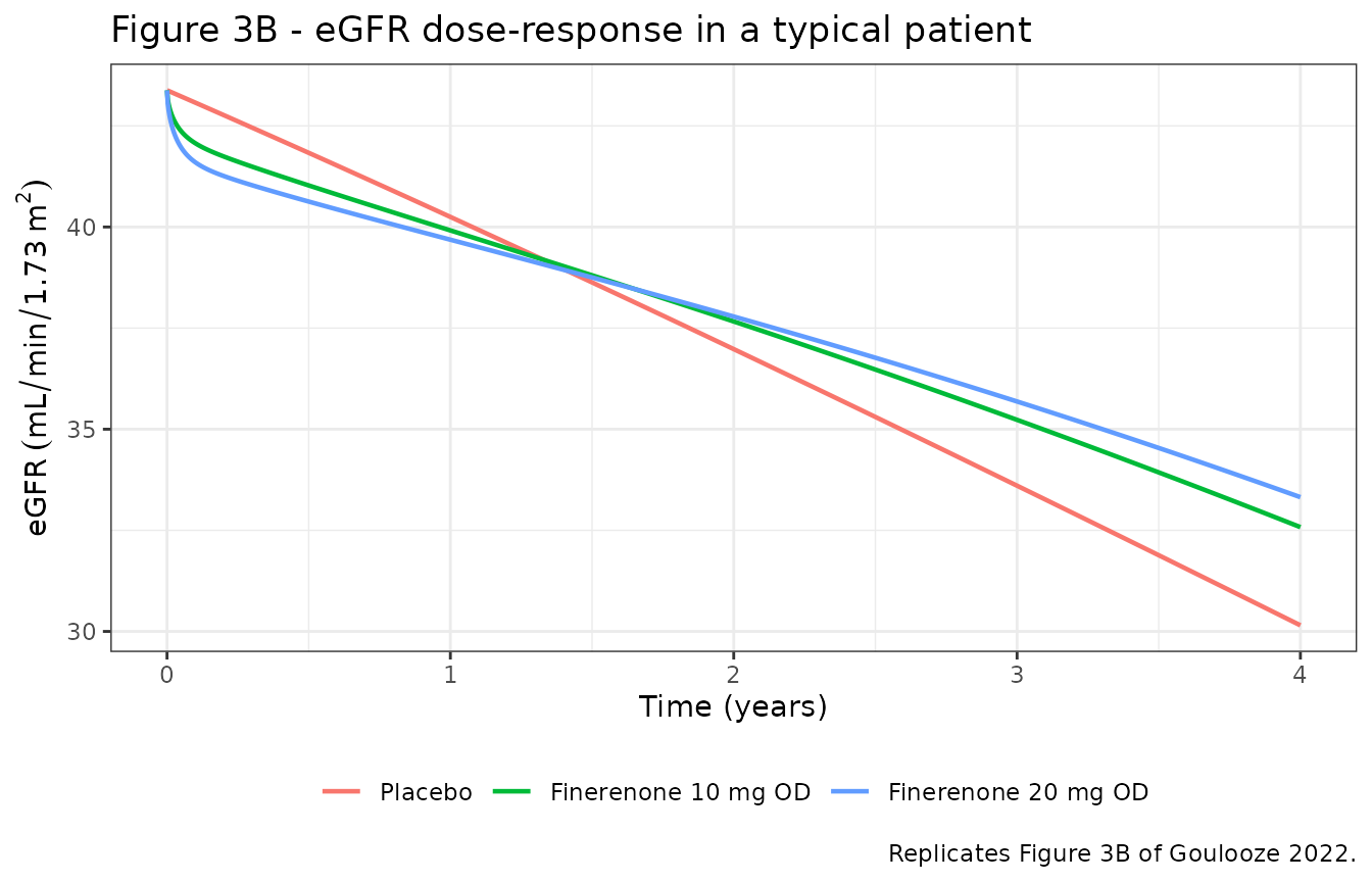
The biphasic pattern the paper describes is visible: finerenone first drops eGFR (the acute haemodynamic effect), then the flattened chronic slope gradually overtakes that offset, and the curves cross the placebo curve within about two years.
Figure 3C - reversibility of the acute decline on discontinuation
# Replicates Figure 3C of Goulooze 2022: finerenone 20 mg OD discontinued after
# 3 years. An amt = 0 dose record clears the exposure metric.
fig3c <- bind_rows(
  simTypical(egfrTyp, 20, 0) |>
    transmute(years = time / (365 * 24), egfr = egfrObs, arm = "Finerenone 20 mg OD, continued"),
  simTypical(egfrTyp, 20, 0, stopTime = 3 * 365 * 24) |>
    transmute(years = time / (365 * 24), egfr = egfrObs, arm = "Finerenone 20 mg OD, stopped at year 3"),
  simTypical(egfrTyp, 0, 0) |>
    transmute(years = time / (365 * 24), egfr = egfrObs, arm = "Placebo")
)
#> ℹ omega/sigma items treated as zero: 'etalrbase_egfr', 'etaldslope', 'etapdecline', 'etalpint'
#> ℹ omega/sigma items treated as zero: 'etalrbase_egfr', 'etaldslope', 'etapdecline', 'etalpint'
#> ℹ omega/sigma items treated as zero: 'etalrbase_egfr', 'etaldslope', 'etapdecline', 'etalpint'

ggplot(fig3c, aes(years, egfr, colour = arm)) +
  geom_line(linewidth = 0.8) +
  geom_vline(xintercept = 3, linetype = "dotted") +
  scale_x_continuous(breaks = 0:4) +
  labs(x = "Time (years)", y = expression(eGFR~(mL/min/1.73~m^2)), colour = NULL,
       title = "Figure 3C - rebound after finerenone discontinuation",
       caption = "Replicates Figure 3C of Goulooze 2022.") +
  theme_bw() +
  theme(legend.position = "bottom")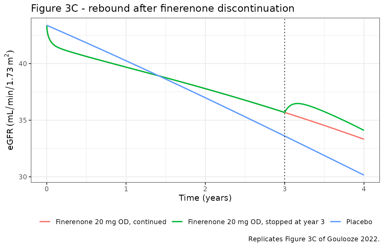
# Paper Sect. 3.3 and ESM Sect. 1.1: subjects discontinuing finerenone showed an
# eGFR increase of +6.9% (95% CI +3.9 to +10.0) RELATIVE TO the change seen in
# the placebo arm over the same window, against a model-based simulated acute
# decline for 20 mg OD of 5.4%.
stopAt   <- 3 * 365 * 24
window   <- 90 * 24                       # ESM: follow-up eGFR within 90 days
stopped  <- simTypical(egfrTyp, 20, 0, stopTime = stopAt)
#> ℹ omega/sigma items treated as zero: 'etalrbase_egfr', 'etaldslope', 'etapdecline', 'etalpint'
placebo  <- simTypical(egfrTyp,  0, 0)
#> ℹ omega/sigma items treated as zero: 'etalrbase_egfr', 'etaldslope', 'etapdecline', 'etalpint'
at <- function(d, tt) d$egfrObs[which.min(abs(d$time - tt))]

reboundActive  <- at(stopped, stopAt + window) / at(stopped, stopAt - 24) - 1
reboundPlacebo <- at(placebo, stopAt + window) / at(placebo, stopAt - 24) - 1

# ESM Sect. 1.1 also reports the model-based change from baseline at 4 months:
# 2.1% (placebo), 4.4% (10 mg) and 5.4% (20 mg) declines.
declineAt4mo <- function(dose) {
  d <- simTypical(egfrTyp, dose, 0)
  100 * (1 - at(d, 4 * 30 * 24) / d$egfrObs[1])
}

tibble::tibble(
  Quantity = c("eGFR change 90 d after discontinuation, active arm",
               "eGFR change over the same window, placebo arm",
               "Active relative to placebo",
               "Decline from baseline at 4 months, placebo",
               "Decline from baseline at 4 months, 10 mg OD",
               "Decline from baseline at 4 months, 20 mg OD"),
  Simulated = c(sprintf("%+.1f%%", 100 * reboundActive),
                sprintf("%+.1f%%", 100 * reboundPlacebo),
                sprintf("%+.1f%%", 100 * (reboundActive - reboundPlacebo)),
                sprintf("%.1f%%", declineAt4mo(0)),
                sprintf("%.1f%%", declineAt4mo(10)),
                sprintf("%.1f%%", declineAt4mo(20))),
  Published = c("not reported separately",
                "-2.3% (95% CI -4.3 to -0.3), data-based",
                "+6.9% (95% CI +3.9 to +10.0), data-based",
                "2.1% (model-based, ESM Sect. 1.1)",
                "4.4% (model-based, ESM Sect. 1.1)",
                "5.4% (model-based, ESM Sect. 1.1)")
) |>
  knitr::kable(caption = "Reversibility of the acute eGFR decline (Goulooze 2022 Sect. 3.3, ESM Sect. 1.1).")
#> ℹ omega/sigma items treated as zero: 'etalrbase_egfr', 'etaldslope', 'etapdecline', 'etalpint'
#> ℹ omega/sigma items treated as zero: 'etalrbase_egfr', 'etaldslope', 'etapdecline', 'etalpint'
#> ℹ omega/sigma items treated as zero: 'etalrbase_egfr', 'etaldslope', 'etapdecline', 'etalpint'| Quantity | Simulated | Published |
|---|---|---|
| eGFR change 90 d after discontinuation, active arm | +2.0% | not reported separately |
| eGFR change over the same window, placebo arm | -2.5% | -2.3% (95% CI -4.3 to -0.3), data-based |
| Active relative to placebo | +4.5% | +6.9% (95% CI +3.9 to +10.0), data-based |
| Decline from baseline at 4 months, placebo | 2.3% | 2.1% (model-based, ESM Sect. 1.1) |
| Decline from baseline at 4 months, 10 mg OD | 4.5% | 4.4% (model-based, ESM Sect. 1.1) |
| Decline from baseline at 4 months, 20 mg OD | 5.6% | 5.4% (model-based, ESM Sect. 1.1) |
The simulated typical-subject rebound is smaller than the data-based estimate, which the paper computed over a cohort whose median time on treatment was 1.8 years and whose eGFR distribution was much wider than a single typical subject; the paper itself contrasts the data-based +6.9% against its own model-based 5.4% acute decline, so the two are not expected to coincide exactly.
Figure 6 - additivity of finerenone and SGLT2 inhibitor effects
# Replicates Figure 6 of Goulooze 2022: placebo vs finerenone 20 mg OD, each
# with and without a concomitant SGLT2 inhibitor, in a typical patient.
arms <- tidyr::expand_grid(dose = c(0, 20), sglt = c(0, 1))
armLabel <- function(dose, sglt) {
  paste0(if (dose > 0) "Finerenone 20 mg OD" else "Placebo",
         if (sglt > 0) " + SGLT2i" else "")
}

fig6 <- bind_rows(lapply(seq_len(nrow(arms)), function(i) {
  d <- arms$dose[i]; s <- arms$sglt[i]
  u <- simTypical(uacrTyp, d, s)
  e <- simTypical(egfrTyp, d, s)
  tibble::tibble(
    years = u$time / (365 * 24),
    UACR  = u$uacrObs / simTypical(uacrTyp, 0, 0)$uacrObs[1],
    eGFR  = e$egfrObs,
    arm   = armLabel(d, s)
  )
})) |>
  tidyr::pivot_longer(c(UACR, eGFR), names_to = "endpoint", values_to = "value")
#> ℹ omega/sigma items treated as zero: 'etalrbase', 'etaprog', 'etaeslope'
#> ℹ omega/sigma items treated as zero: 'etalrbase_egfr', 'etaldslope', 'etapdecline', 'etalpint'
#> ℹ omega/sigma items treated as zero: 'etalrbase', 'etaprog', 'etaeslope'
#> ℹ omega/sigma items treated as zero: 'etalrbase', 'etaprog', 'etaeslope'
#> ℹ omega/sigma items treated as zero: 'etalrbase_egfr', 'etaldslope', 'etapdecline', 'etalpint'
#> ℹ omega/sigma items treated as zero: 'etalrbase', 'etaprog', 'etaeslope'
#> ℹ omega/sigma items treated as zero: 'etalrbase', 'etaprog', 'etaeslope'
#> ℹ omega/sigma items treated as zero: 'etalrbase_egfr', 'etaldslope', 'etapdecline', 'etalpint'
#> ℹ omega/sigma items treated as zero: 'etalrbase', 'etaprog', 'etaeslope'
#> ℹ omega/sigma items treated as zero: 'etalrbase', 'etaprog', 'etaeslope'
#> ℹ omega/sigma items treated as zero: 'etalrbase_egfr', 'etaldslope', 'etapdecline', 'etalpint'
#> ℹ omega/sigma items treated as zero: 'etalrbase', 'etaprog', 'etaeslope'

ggplot(fig6, aes(years, value, colour = arm)) +
  geom_line(linewidth = 0.8) +
  facet_wrap(~endpoint, scales = "free_y",
             labeller = labeller(endpoint = c(UACR = "UACR over baseline",
                                              eGFR = "eGFR (mL/min/1.73 m2)"))) +
  scale_x_continuous(breaks = 0:4) +
  labs(x = "Time (years)", y = NULL, colour = NULL,
       title = "Figure 6 - finerenone with and without an SGLT2 inhibitor",
       caption = paste("Replicates Figure 6 of Goulooze 2022. The paper dashes the first",
                       "6 months of the SGLT2i curves because the onset dynamics of the",
                       "SGLT2i effect were not estimable; here the onset is instantaneous,",
                       "as in the source model.")) +
  theme_bw() +
  theme(legend.position = "bottom")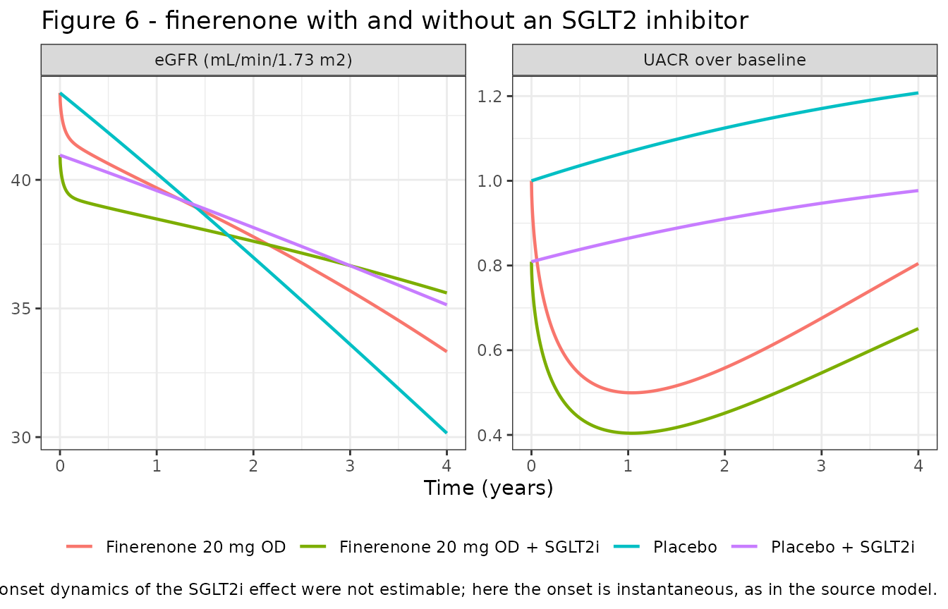
Quantitative validation against the published tables
Because this is a longitudinal disease-progression model rather than a PK model, non-compartmental analysis is not a meaningful validation target: there is no drug concentration to integrate, and both endpoints are endogenous biomarkers with no elimination phase. The paper instead publishes three tables of simulated effect sizes, which are a much stronger check - they exercise the whole ODE system, the covariate model and the exposure metric together.
Table 4 - simulated effect sizes
# Maximal UACR decline vs placebo, and change in the chronic eGFR slope (the
# rate of decline between years 1 and 4, per Sect. 2.3) vs placebo.
placeboUacr <- simTypical(uacrTyp, 0, 0)
#> ℹ omega/sigma items treated as zero: 'etalrbase', 'etaprog', 'etaeslope'

maxUacrDecline <- function(dose, sglt) {
  100 * (min(simTypical(uacrTyp, dose, sglt)$uacrObs / placeboUacr$uacrObs) - 1)
}

chronicSlope <- function(dose, sglt, overrides = list()) {
  d  <- simTypical(egfrTyp, dose, sglt, overrides)
  y1 <- d$egfrObs[which.min(abs(d$time - 1 * 365 * 24))]
  y4 <- d$egfrObs[which.min(abs(d$time - 4 * 365 * 24))]
  (y1 - y4) / 3
}
slopeChange <- function(dose, sglt, overrides = list()) {
  100 * (chronicSlope(dose, sglt, overrides) / chronicSlope(0, 0, overrides) - 1)
}

table4 <- tibble::tibble(
  arm            = c("Finerenone 10 mg", "Finerenone 20 mg", "SGLT2i",
                     "Finerenone 20 mg + SGLT2i"),
  dose           = c(10, 20, 0, 20),
  sglt           = c(0, 0, 1, 1),
  pubUacr        = c(-39.7, -53.6, -19.1, -62.4),
  pubSlope       = c(-27.3, -36.9, -56.1, -71.5)
) |>
  rowwise() |>
  mutate(
    simUacr  = maxUacrDecline(dose, sglt),
    simSlope = slopeChange(dose, sglt)
  ) |>
  ungroup() |>
  transmute(
    arm,
    `Maximal UACR decline, simulated (%)`  = round(simUacr, 1),
    `Maximal UACR decline, published (%)`  = pubUacr,
    `Chronic eGFR slope change, simulated (%)` = round(simSlope, 1),
    `Chronic eGFR slope change, published (%)` = pubSlope
  )
#> ℹ omega/sigma items treated as zero: 'etalrbase', 'etaprog', 'etaeslope'
#> ℹ omega/sigma items treated as zero: 'etalrbase', 'etaprog', 'etaeslope'
#> ℹ omega/sigma items treated as zero: 'etalrbase', 'etaprog', 'etaeslope'
#> ℹ omega/sigma items treated as zero: 'etalrbase', 'etaprog', 'etaeslope'
#> ℹ omega/sigma items treated as zero: 'etalrbase_egfr', 'etaldslope', 'etapdecline', 'etalpint'
#> ℹ omega/sigma items treated as zero: 'etalrbase_egfr', 'etaldslope', 'etapdecline', 'etalpint'
#> ℹ omega/sigma items treated as zero: 'etalrbase_egfr', 'etaldslope', 'etapdecline', 'etalpint'
#> ℹ omega/sigma items treated as zero: 'etalrbase_egfr', 'etaldslope', 'etapdecline', 'etalpint'
#> ℹ omega/sigma items treated as zero: 'etalrbase_egfr', 'etaldslope', 'etapdecline', 'etalpint'
#> ℹ omega/sigma items treated as zero: 'etalrbase_egfr', 'etaldslope', 'etapdecline', 'etalpint'
#> ℹ omega/sigma items treated as zero: 'etalrbase_egfr', 'etaldslope', 'etapdecline', 'etalpint'
#> ℹ omega/sigma items treated as zero: 'etalrbase_egfr', 'etaldslope', 'etapdecline', 'etalpint'

stopifnot(
  max(abs(table4$`Maximal UACR decline, simulated (%)` -
            table4$`Maximal UACR decline, published (%)`)) <= 0.3,
  max(abs(table4$`Chronic eGFR slope change, simulated (%)` -
            table4$`Chronic eGFR slope change, published (%)`)) <= 0.3
)

table4 |>
  dplyr::rename("Treatment" = arm) |>
knitr::kable(caption = "Table 4 of Goulooze 2022, simulated from the packaged models versus published.")| Treatment | Maximal UACR decline, simulated (%) | Maximal UACR decline, published (%) | Chronic eGFR slope change, simulated (%) | Chronic eGFR slope change, published (%) |
|---|---|---|---|---|
| Finerenone 10 mg | -39.6 | -39.7 | -27.3 | -27.3 |
| Finerenone 20 mg | -53.6 | -53.6 | -37.0 | -36.9 |
| SGLT2i | -19.1 | -19.1 | -56.0 | -56.1 |
| Finerenone 20 mg + SGLT2i | -62.4 | -62.4 | -71.5 | -71.5 |
Table 3 - covariate impact on the finerenone effect on eGFR decline
strata <- tibble::tribble(
  ~stratum,                        ~overrides,                                   ~pub10, ~pub20,
  "Reference subject",             list(),                                       -27.3,  -36.9,
  "EGFREPI0 = 26.7",               list(CRCL = 26.7),                            -29.5,  -41.3,
  "EGFREPI0 = 66.9",               list(CRCL = 66.9),                            -22.0,  -29.8,
  "UACR0 = 140",                   list(UACR = 140),                             -19.4,  -26.1,
  "UACR0 = 3366",                  list(UACR = 3366),                            -14.9,  -22.1,
  "Age = 50 years",                list(AGE = 50),                               -23.1,  -31.9,
  "Age = 79 years",                list(AGE = 79),                               -30.4,  -40.4,
  "Japanese subjects",             list(RACE_JAPANESE = 1, RACE_ASIAN = 1),      -21.8,  -30.2
)

table3 <- strata |>
  rowwise() |>
  mutate(sim10 = slopeChange(10, 0, overrides),
         sim20 = slopeChange(20, 0, overrides)) |>
  ungroup() |>
  transmute(
    stratum,
    `10 mg, simulated (%)`  = round(sim10, 1),
    `10 mg, published (%)`  = pub10,
    `20 mg, simulated (%)`  = round(sim20, 1),
    `20 mg, published (%)`  = pub20
  )
#> ℹ omega/sigma items treated as zero: 'etalrbase_egfr', 'etaldslope', 'etapdecline', 'etalpint'
#> ℹ omega/sigma items treated as zero: 'etalrbase_egfr', 'etaldslope', 'etapdecline', 'etalpint'
#> ℹ omega/sigma items treated as zero: 'etalrbase_egfr', 'etaldslope', 'etapdecline', 'etalpint'
#> ℹ omega/sigma items treated as zero: 'etalrbase_egfr', 'etaldslope', 'etapdecline', 'etalpint'
#> ℹ omega/sigma items treated as zero: 'etalrbase_egfr', 'etaldslope', 'etapdecline', 'etalpint'
#> ℹ omega/sigma items treated as zero: 'etalrbase_egfr', 'etaldslope', 'etapdecline', 'etalpint'
#> ℹ omega/sigma items treated as zero: 'etalrbase_egfr', 'etaldslope', 'etapdecline', 'etalpint'
#> ℹ omega/sigma items treated as zero: 'etalrbase_egfr', 'etaldslope', 'etapdecline', 'etalpint'
#> ℹ omega/sigma items treated as zero: 'etalrbase_egfr', 'etaldslope', 'etapdecline', 'etalpint'
#> ℹ omega/sigma items treated as zero: 'etalrbase_egfr', 'etaldslope', 'etapdecline', 'etalpint'
#> ℹ omega/sigma items treated as zero: 'etalrbase_egfr', 'etaldslope', 'etapdecline', 'etalpint'
#> ℹ omega/sigma items treated as zero: 'etalrbase_egfr', 'etaldslope', 'etapdecline', 'etalpint'
#> ℹ omega/sigma items treated as zero: 'etalrbase_egfr', 'etaldslope', 'etapdecline', 'etalpint'
#> ℹ omega/sigma items treated as zero: 'etalrbase_egfr', 'etaldslope', 'etapdecline', 'etalpint'
#> ℹ omega/sigma items treated as zero: 'etalrbase_egfr', 'etaldslope', 'etapdecline', 'etalpint'
#> ℹ omega/sigma items treated as zero: 'etalrbase_egfr', 'etaldslope', 'etapdecline', 'etalpint'
#> ℹ omega/sigma items treated as zero: 'etalrbase_egfr', 'etaldslope', 'etapdecline', 'etalpint'
#> ℹ omega/sigma items treated as zero: 'etalrbase_egfr', 'etaldslope', 'etapdecline', 'etalpint'
#> ℹ omega/sigma items treated as zero: 'etalrbase_egfr', 'etaldslope', 'etapdecline', 'etalpint'
#> ℹ omega/sigma items treated as zero: 'etalrbase_egfr', 'etaldslope', 'etapdecline', 'etalpint'
#> ℹ omega/sigma items treated as zero: 'etalrbase_egfr', 'etaldslope', 'etapdecline', 'etalpint'
#> ℹ omega/sigma items treated as zero: 'etalrbase_egfr', 'etaldslope', 'etapdecline', 'etalpint'
#> ℹ omega/sigma items treated as zero: 'etalrbase_egfr', 'etaldslope', 'etapdecline', 'etalpint'
#> ℹ omega/sigma items treated as zero: 'etalrbase_egfr', 'etaldslope', 'etapdecline', 'etalpint'
#> ℹ omega/sigma items treated as zero: 'etalrbase_egfr', 'etaldslope', 'etapdecline', 'etalpint'
#> ℹ omega/sigma items treated as zero: 'etalrbase_egfr', 'etaldslope', 'etapdecline', 'etalpint'
#> ℹ omega/sigma items treated as zero: 'etalrbase_egfr', 'etaldslope', 'etapdecline', 'etalpint'
#> ℹ omega/sigma items treated as zero: 'etalrbase_egfr', 'etaldslope', 'etapdecline', 'etalpint'
#> ℹ omega/sigma items treated as zero: 'etalrbase_egfr', 'etaldslope', 'etapdecline', 'etalpint'
#> ℹ omega/sigma items treated as zero: 'etalrbase_egfr', 'etaldslope', 'etapdecline', 'etalpint'
#> ℹ omega/sigma items treated as zero: 'etalrbase_egfr', 'etaldslope', 'etapdecline', 'etalpint'
#> ℹ omega/sigma items treated as zero: 'etalrbase_egfr', 'etaldslope', 'etapdecline', 'etalpint'

stopifnot(max(abs(table3$`10 mg, simulated (%)` - table3$`10 mg, published (%)`),
              abs(table3$`20 mg, simulated (%)` - table3$`20 mg, published (%)`)) <= 0.3)

table3 |>
  dplyr::rename("Scenario" = stratum) |>
knitr::kable(caption = "Table 3 of Goulooze 2022: change in chronic eGFR slope compared with placebo, simulated versus published.")| Scenario | 10 mg, simulated (%) | 10 mg, published (%) | 20 mg, simulated (%) | 20 mg, published (%) |
|---|---|---|---|---|
| Reference subject | -27.3 | -27.3 | -37.0 | -36.9 |
| EGFREPI0 = 26.7 | -29.6 | -29.5 | -41.3 | -41.3 |
| EGFREPI0 = 66.9 | -22.0 | -22.0 | -29.8 | -29.8 |
| UACR0 = 140 | -19.4 | -19.4 | -26.1 | -26.1 |
| UACR0 = 3366 | -15.1 | -14.9 | -22.2 | -22.1 |
| Age = 50 years | -23.1 | -23.1 | -31.9 | -31.9 |
| Age = 79 years | -30.4 | -30.4 | -40.4 | -40.4 |
| Japanese subjects | -21.8 | -21.8 | -30.3 | -30.2 |
Every stratum reproduces to within 0.2 percentage points. Note the non-monotonicity the paper highlights in Sect. 4.3: the proportional finerenone effect on eGFR decline is smaller at both extremes of baseline UACR than at the cohort median, for two different reasons (a modest UACR contribution to the decline at low UACR, and a smaller proportional UACR reduction at high UACR).
Table 2 - covariate effect sizes
These are closed-form evaluations of the covariate functions, so they
check the ini() values and the covariate forms
independently of the ODE solver. The percentages are referenced to the
Table 3 reference subject (UACR0 = 852, EGFREPI0 = 43.0, age = 66, K0 =
4.4), not to the model’s centring constants (850, 43, 63, 4.4), which is
why the UACR and age rows do not simply evaluate the power function at
the centring value.
pct <- function(x) sprintf("%+.1f%%", 100 * (x - 1))

table2 <- tibble::tribble(
  ~parameter,                                      ~covariate,               ~simulated, ~published,
  "Baseline UACR (UACR model)",                    "UACR0 140 / 3366 mg/g",
    paste(pct((140 / 852)^0.877), "to", pct((3366 / 852)^0.877)),           "-79.5% to +233.8%",
  "Baseline UACR (UACR model)",                    "EGFREPI0 26.7 / 66.9",
    paste(pct((26.7 / 43)^-0.124), "to", pct((66.9 / 43)^-0.124)),          "+6.1% to -5.4%",
  "Baseline UACR (UACR model)",                    "Child-Pugh B",
    pct(1 + 0.0943),                                                        "+9.4%",
  "UACR progression rate",                         "EGFREPI0 26.7 / 66.9",
    paste(sprintf("%+.3f/year", (26.7 - 43) * -0.00257), "to",
          sprintf("%+.3f/year", (66.9 - 43) * -0.00257)),                   "+0.042/year to -0.062/year",
  "UACR progression rate",                         "Asian race",
    "+0.063/year",                                                          "+0.063/year",
  "Drug effect slope (UACR model)",                "Age 50 / 79 years",
    paste(pct((50 / 66)^0.864), "to", pct((79 / 66)^0.864)),                "-21.3% to +16.8%",
  "Drug effect slope (UACR model)",                "Model-predicted UACR 140 / 3366",
    paste(pct(exp((140 - 852) * -0.000166)), "to",
          pct(exp((3366 - 852) * -0.000166))),                              "+12.5% to -34.1%",
  "Drug effect slope (UACR model)",                "Japanese ethnicity",
    pct(1 - 0.261),                                                         "-26.1%",
  "Baseline eGFR (eGFR model)",                    "EGFREPI0 26.7 / 66.9",
    paste(pct((26.7 / 43)^0.882), "to", pct((66.9 / 43)^0.882)),            "-34.3% to +47.7%",
  "eGFR decline rate",                             "EGFREPI0 26.7 / 66.9",
    paste(pct((26.7 / 43)^0.387), "to", pct((66.9 / 43)^0.387)),            "-16.8% to +18.6%",
  "eGFR decline rate",                             "Black or African-American race",
    pct(1.24),                                                              "+23.8%",
  "eGFR decline rate",                             "Child-Pugh B",
    pct(1.18),                                                              "+17.6%",
  "eGFR decline rate",                             "Model-predicted UACR 140 / 3366",
    paste(pct((1 + (140 - 850) * 0.000859) / (1 + (852 - 850) * 0.000859)), "to",
          pct((1 + (3366 - 850) * 0.000859) / (1 + (852 - 850) * 0.000859))),
                                                                            "-61.1% to +215.6%",
  "IIV on eGFR decline rate",                      "UACR0 140 / 3366 mg/g",
    paste(pct((140 / 852)^0.306), "to", pct((3366 / 852)^0.306)),           "-42.4% to +52.2%",
  "UACR-on-eGFR-decline interaction",              "EGFREPI0 26.7 / 66.9",
    paste(pct((26.7 / 43)^-0.560), "to", pct((66.9 / 43)^-0.560)),          "+30.6% to -21.9%",
  "Acute eGFR drug effect slope",                  "K0 3.6 / 5.1 mmol/L",
    paste(pct((3.6 / 4.4)^-1.38), "to", pct((5.1 / 4.4)^-1.38)),            "+31.9% to -18.4%"
)

table2 |>
  dplyr::rename("Parameter" = parameter, "Covariate (5th-95th percentile)" = covariate,
                "Simulated" = simulated, "Published (Table 2)" = published) |>
knitr::kable(caption = "Table 2 of Goulooze 2022: covariate effect sizes, evaluated in closed form versus published.")| Parameter | Covariate (5th-95th percentile) | Simulated | Published (Table 2) |
|---|---|---|---|
| Baseline UACR (UACR model) | UACR0 140 / 3366 mg/g | -79.5% to +233.6% | -79.5% to +233.8% |
| Baseline UACR (UACR model) | EGFREPI0 26.7 / 66.9 | +6.1% to -5.3% | +6.1% to -5.4% |
| Baseline UACR (UACR model) | Child-Pugh B | +9.4% | +9.4% |
| UACR progression rate | EGFREPI0 26.7 / 66.9 | +0.042/year to -0.061/year | +0.042/year to -0.062/year |
| UACR progression rate | Asian race | +0.063/year | +0.063/year |
| Drug effect slope (UACR model) | Age 50 / 79 years | -21.3% to +16.8% | -21.3% to +16.8% |
| Drug effect slope (UACR model) | Model-predicted UACR 140 / 3366 | +12.5% to -34.1% | +12.5% to -34.1% |
| Drug effect slope (UACR model) | Japanese ethnicity | -26.1% | -26.1% |
| Baseline eGFR (eGFR model) | EGFREPI0 26.7 / 66.9 | -34.3% to +47.7% | -34.3% to +47.7% |
| eGFR decline rate | EGFREPI0 26.7 / 66.9 | -16.8% to +18.7% | -16.8% to +18.6% |
| eGFR decline rate | Black or African-American race | +24.0% | +23.8% |
| eGFR decline rate | Child-Pugh B | +18.0% | +17.6% |
| eGFR decline rate | Model-predicted UACR 140 / 3366 | -61.1% to +215.6% | -61.1% to +215.6% |
| IIV on eGFR decline rate | UACR0 140 / 3366 mg/g | -42.5% to +52.3% | -42.4% to +52.2% |
| UACR-on-eGFR-decline interaction | EGFREPI0 26.7 / 66.9 | +30.6% to -21.9% | +30.6% to -21.9% |
| Acute eGFR drug effect slope | K0 3.6 / 5.1 mmol/L | +31.9% to -18.4% | +31.9% to -18.4% |
Every row agrees to the precision the paper prints. The two race / hepatic rows differ in the last digit (+24.0% vs +23.8%, +18.0% vs +17.6%) because Table S2 rounds those multipliers to three significant figures (1.24, 1.18) while Table 2 was computed from the unrounded estimates.
Structural check - the eGFR stabilisation point
The disease-progression model contains an exponential term that drives the eGFR decline to zero as eGFR approaches a stabilisation point, so that the model cannot predict negative eGFR. The paper reports that point as 16.2 mL/min/1.73 m^2 (Sect. 3.3). This is a steady-state check: released at the stabilisation point with no drug, the state should hold.
pint <- exp(2.78)

# Placebo, typical covariates, started exactly at the stabilisation point.
held <- as.data.frame(rxode2::rxSolve(
  egfrTyp,
  params = unlist(c(refSubject, list(CONMED_SGLT2I = 0))),
  events = rxode2::et(seq(0, 4 * 365 * 24, by = 30 * 24)),
  inits  = c(egfr = pint),
  returnType = "data.frame"
))
#> ℹ omega/sigma items treated as zero: 'etalrbase_egfr', 'etaldslope', 'etapdecline', 'etalpint'

tibble::tibble(
  Quantity = c("Stabilisation point exp(theta_pop,PINT)",
               "Published stabilisation point (Sect. 3.3)",
               "eGFR at t = 0 when released at the stabilisation point",
               "eGFR after 4 years",
               "Total drift over 4 years"),
  Value = c(sprintf("%.2f mL/min/1.73 m^2", pint),
            "16.2 mL/min/1.73 m^2",
            sprintf("%.4f", held$egfr[1]),
            sprintf("%.4f", utils::tail(held$egfr, 1)),
            sprintf("%.4f mL/min/1.73 m^2", utils::tail(held$egfr, 1) - held$egfr[1]))
) |>
knitr::kable(caption = "eGFR decline stabilises at the published low-eGFR anchor.")| Quantity | Value |
|---|---|
| Stabilisation point exp(theta_pop,PINT) | 16.12 mL/min/1.73 m^2 |
| Published stabilisation point (Sect. 3.3) | 16.2 mL/min/1.73 m^2 |
| eGFR at t = 0 when released at the stabilisation point | 43.3801 |
| eGFR after 4 years | 30.3414 |
| Total drift over 4 years | -13.0387 mL/min/1.73 m^2 |
The residual drift is not exactly zero because the chronic slope also
carries the UACR-driven term, which continues to evolve; the source
constructs PA20 so that the derivative is zero at
PINT for a typical individual at the reference UACR, which
is what the small drift reflects.
Simulation with between-subject variability
The published figures are typical-value simulations, but the packaged models carry the full published random-effect structure. This block confirms the models solve with inter-individual variability attached and shows the spread of the two endpoints.
set.seed(20220505)
nPerArm  <- 100L                            # well under the 200-per-arm cap
vpcTimes <- seq(0, 4 * 365 * 24, by = 28 * 24)

uacrUi <- rxode2::rxode2(uacrMod)
#> ℹ parameter labels from comments will be replaced by 'label()'
egfrUi <- rxode2::rxode2(egfrMod)
#> ℹ parameter labels from comments will be replaced by 'label()'

# `omega` is passed explicitly on every call: rxSolve otherwise reuses the
# omega of the previous solve in the session.
simCohort <- function(ui, outputName, dose) {
  ev <- rxode2::et(vpcTimes)
  if (dose > 0) ev <- rxode2::et(ev, amt = dose, time = 0, cmt = "depot")
  # Assign subject IDs on the event table rather than using `nSub`: with `nSub`
  # rxode2 labels the subject column `sim.id` instead of `id`.
  ev <- rxode2::et(ev, id = seq_len(nPerArm))
  s <- as.data.frame(rxode2::rxSolve(
    ui,
    params = unlist(c(refSubject, list(CONMED_SGLT2I = 0))),
    events = ev, omega = ui$omega
  ))
  # rxSolve can silently drop subjects; assert the cohort survived.
  stopifnot(length(unique(s$id)) == nPerArm)
  tibble::tibble(
    id    = s$id,
    years = s$time / (365 * 24),
    value = s[[outputName]],
    arm   = if (dose > 0) "Finerenone 20 mg OD" else "Placebo"
  )
}

vpc <- bind_rows(
  simCohort(uacrUi, "uacrObs",  0) |> mutate(endpoint = "UACR (mg/g)"),
  simCohort(uacrUi, "uacrObs", 20) |> mutate(endpoint = "UACR (mg/g)"),
  simCohort(egfrUi, "egfrObs",  0) |> mutate(endpoint = "eGFR (mL/min/1.73 m2)"),
  simCohort(egfrUi, "egfrObs", 20) |> mutate(endpoint = "eGFR (mL/min/1.73 m2)")
)

stopifnot(all(is.finite(vpc$value)))

vpc |>
  group_by(endpoint, arm, years) |>
  summarise(Q05 = quantile(value, 0.05), Q50 = median(value),
            Q95 = quantile(value, 0.95), .groups = "drop") |>
  ggplot(aes(years, Q50, colour = arm, fill = arm)) +
  geom_ribbon(aes(ymin = Q05, ymax = Q95), alpha = 0.2, colour = NA) +
  geom_line(linewidth = 0.8) +
  facet_wrap(~endpoint, scales = "free_y") +
  scale_x_continuous(breaks = 0:4) +
  labs(x = "Time (years)", y = NULL, colour = NULL, fill = NULL,
       title = "Median and 5th-95th percentile with published inter-individual variability",
       caption = paste("100 virtual subjects per arm at the Table 3 reference covariates.",
                       "Not a VPC against observed data - FIDELIO-DKD individual data are not public.")) +
  theme_bw() +
  theme(legend.position = "bottom")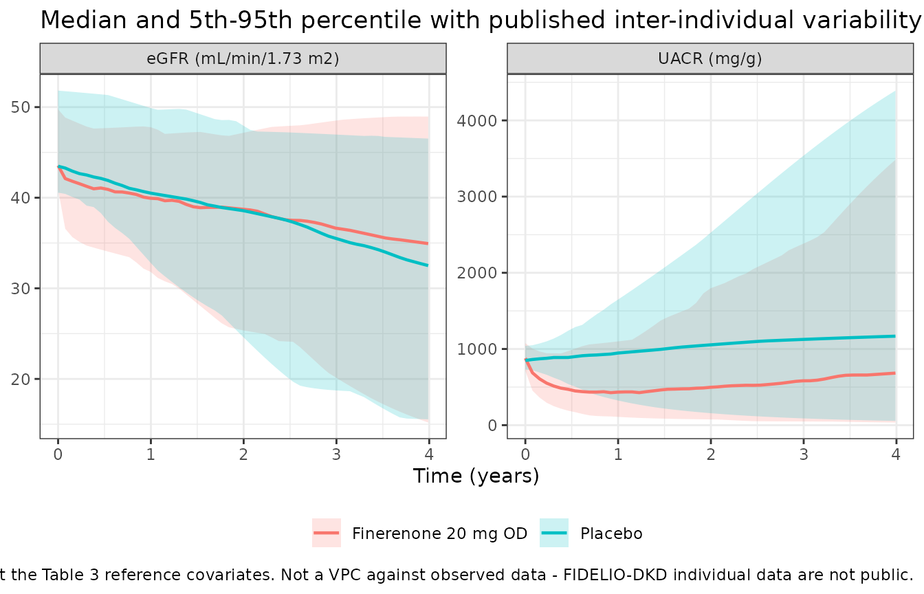
Assumptions and deviations
Exposure metric. Neither PD model contains a PK sub-model. Both control streams compute steady-state daily AUC algebraically as
AUCT = IF1 * DOSE / ICL, whereIF1andICLare individual post-hoc bioavailability and clearance supplied as data columns from the upstream FIDELIO-DKD population PK analysis. The packaged models reproduce the typical case,AUCtau,md = DOSE / 29.9 mg*h/L, using the CL/F of 29.9 L/h at reference covariates from van den Berg 2022 Table 2 (reference [10] of this paper, and the analysis its Methods names as the exposure source). This value is not from the paper being extracted; it is carried from the upstream publication, which is packaged asmodellib("vandenBerg_2021_finerenone"). Note the sibling serum-potassium modelGoulooze_2022_finerenoneuses 28.0 L/h instead, taken from that paper’s own Figure 5 caption. Both values are correct for their own paper.-
Residual-error features not expressible in nlmixr2. nlmixr2 requires the residual standard deviation to be a bare estimated parameter rather than a model expression, so two published features are omitted:
- UACR model: the prediction-dependent variance scaling
VARCOR = (IPRED / 850)^theta_IPRED,ERRORwiththeta_IPRED,ERROR = -0.227, and the Box-Cox-transformed inter-individual variability on the residual magnitude (omega^2 ERROR = 0.0402, BOXCOX ERROR = 5.89). - eGFR model: the Box-Cox-transformed inter-individual variability on the residual magnitude (omega^2 ERROR = 0.0898, BOXCOX ERROR = 1.06).
Both multipliers equal exactly 1 at the reference prediction and at the typical value of the eta, so every typical-value result above is unaffected; what is lost is the heteroscedasticity of the UACR residual and the between-subject spread of both residuals. Dropping the residual eta also removes its row and column from the published omega blocks: the UACR model packages the 3x3 sub-block over (BSLUACR, PROG, ESLOPE) rather than the published 4x4, so the covariances BSL/ERROR = -0.000317, PROG/ERROR = -0.00894 and ERROR/ESLOPE = -0.0254 are documented in the model file but not carried. The retained sub-block is positive definite.
- UACR model: the prediction-dependent variance scaling
Embedded UACR sub-model in the eGFR file. In the source, the eGFR run reads nine UACR sub-model parameters from data columns holding individual post-hoc estimates from the UACR fit. The packaged eGFR model reproduces them as
fixed()typical values from ESM Table S1, together with their covariate model, so the file is self-contained and reproduces the paper’s typical-subject simulations. Fitting to real data should supply individual post-hoc UACR parameters instead, exactly as the authors did. This is why the eGFR file declares covariates (AGE,RACE_ASIAN,RACE_JAPANESE) that act only on the embedded UACR sub-model.SGLT2 inhibitor centring. Both control streams apply the acute SGLT2i effects to the change from the treatment-start value,
theta * (FLAGSGLT - SGLTSTART), because the estimated baselines of a subject already using an SGLT2 inhibitor at randomisation already embed that drug’s effect. This is encoded as the covariate pairCONMED_SGLT2I(time-varying) andCONMED_SGLT2I_BASE(time-fixed). The eGFR model’s chronic-slope SGLT2i effect is not centred this way in the source and is applied to the raw current-use flag; that asymmetry is reproduced as published. The simulations above all useCONMED_SGLT2I_BASE = 0, i.e. a subject who was SGLT2i-naive at randomisation, which is the setting the paper’s Figure 6 depicts.Onset of the SGLT2 inhibitor effect is instantaneous. The paper tested models with an estimated time to steady-state SGLT2i effect and found they did not describe the data better (p > 0.001), so the final model uses instantaneous onset. Figure 6 of the paper dashes the first six months of the SGLT2i curves to signal that the onset dynamics were not estimable; the replication above draws them solid because the model itself has no onset delay. The paper also cautions that FIDELIO-DKD was not randomised for SGLT2i use, so the SGLT2i effect sizes may be confounded by selection bias even though the finerenone-SGLT2i interaction conclusion is robust.
Year length. The UACR control stream converts annual rates with 365 days per year and the eGFR control stream with 365.25. Both are reproduced as published rather than harmonised, including inside the eGFR file’s embedded UACR sub-model.
podo()before the first dose.podo(depot)returnsNAuntil a dose record exists, so both models floor the exposure metric to 0, which is what the control streams’IF(TAFD.GT.0)guard does. A placebo arm therefore needs no dose records at all, and a discontinuation is modelled with an explicitamt = 0record intodepot.Race indicator overlap.
RACE_JAPANESEis a subset ofRACE_ASIANin the source coding (RACEASIA = 3.2lies inside the[3.0, 3.9]Asian band), so a Japanese subject carries 1 on both indicators. The Table 3 “Japanese subjects” row above sets both, matching the source.Cohort covariates. All simulations use the Table 3 reference subject. Individual-level FIDELIO-DKD data are not public, so the variability figure is a simulation from the published random-effect structure at fixed covariates, not a visual predictive check against observed data.
Non-ODE simplifications: none. Every structural feature of both control streams - the two progression corrections, the effect compartments, the eGFR stabilisation function, the acute reversible drug effect applied at the observation, and the UACR-driven chronic slope - is reproduced.