YH12852 and gastric emptying (Kim 2021)
Source:vignettes/articles/Kim_2021_YH12852.Rmd
Kim_2021_YH12852.RmdModel and source
- Citation: Kim S, Lee HA, Jang SB, Lee H. A population pharmacokinetic-pharmacodynamic model of YH12852, a highly selective 5-hydroxytryptamine 4 receptor agonist, in healthy subjects and patients with functional constipation. CPT Pharmacometrics Syst Pharmacol. 2021;10(8):902-913. doi:10.1002/psp4.12664
- Description: Joint population PK-PD model of the 5-HT4 receptor agonist YH12852 in healthy adults and adults with functional constipation (Kim 2021). The PK is a two-compartment model with first-order absorption, body weight on the peripheral volume, and between-occasion variability on CL/F, V2/F and Ka. The prokinetic effect is a semi-mechanistic three-compartment model of the 13C-Spirulina gastric emptying breath test (GEBT). 13C in the test meal leaves the stomach at rate (K45 + SLP * Cc), and the fraction FC13 is absorbed into the systemic circulation. It then moves to the lung (K56) and is exhaled (Kout = K56). The observed kPCD is the per-minute percent of the 13C dose exhaled, multiplied by 1000. Baseline gastric emptying t10 scales the drug slope SLP.
- Article: https://doi.org/10.1002/psp4.12664 (open access, PMC8376136)
YH12852 is a highly selective 5-HT4 receptor agonist developed for functional constipation. Kim 2021 fitted its plasma PK and its prokinetic effect jointly. The prokinetic effect was measured with the 13C-Spirulina gastric emptying breath test (GEBT). The GEBT endpoint is kPCD, the per-minute percent of the 13C dose exhaled, multiplied by 1000.
The PD part is a small mass-balance model of the 13C label (Kim 2021 Equations 1-4, Figure 1b):
| State | Paper name | Meaning | Out-flow |
|---|---|---|---|
stomach |
compartment 4 (GI tract) | 13C still in the test meal |
(K45 + SLP * Cc); fraction FC13 goes on to
the blood |
c13_blood |
compartment 5 | absorbed 13C in the systemic circulation | K56 |
c13_lung |
compartment 6 | 13C in the lung |
Kout (= K56) to exhaled air |
Each test meal is a bolus of 100,000 kPCD units into
stomach (100 % of the dose x 1000). The observation is
kpcd = Kout * c13_lung / 60, where the /60
converts the per-hour rate constant to the per-minute kPCD. YH12852 adds
a linear term SLP * Cc to the stomach emptying rate
K45. SLP scales with baseline gastric emptying t10 as
(t10 / 30)^3.57: subjects whose stomachs empty slowly at
baseline respond more.
The paper also fitted an empirical Ghoos model (Equation 5, Table S2) and rejected it in favour of this semi-mechanistic model. Only the final model is packaged.
Population
Kim 2021 used data from one randomized, double-blind, placebo-controlled phase I/IIa trial (NCT02538367) in Seoul. The final data set had 1287 plasma concentrations from 49 subjects and 196 kPCD values from 14 subjects (Kim 2021 Results; Table 2):
- The multiple-dose (MD) cohort (N = 35 in the analysis) received 0.3, 0.5, 1, 2 or 3 mg once daily for 14 days. Seventeen of these subjects had functional constipation by the Rome III criteria. The rest were healthy subjects reporting 3 or fewer spontaneous bowel movements per week.
- The multiple-low-dose (MLD) cohort (N = 14) was all healthy and received 0.05 or 0.1 mg once daily for 14 days. Only this cohort had the GEBT, at baseline and on Day 7.
- 71.4 % were women, and the mean age was 27.3 years (range 19-53). Mean weight was 60.4 kg (MD) and 58.2 kg (MLD), with a range of 45.9-78.8 kg.
- MLD baseline t10 was 30.3 +/- 15.5 min (range 11.1-59.4 min).
The same information is available programmatically via
readModelDb("Kim_2021_YH12852")()$population.
Source trace
Every value below also carries an in-file comment in
inst/modeldb/specificDrugs/Kim_2021_YH12852.R. “Control
stream” means the NONMEM code the authors published as Supplementary
Method 2.
| Equation / parameter | Value | Source location |
|---|---|---|
lcl (CL/F) |
88.8 L/h | Table 1 |
lvc (V2/F) |
1380.2 L | Table 1 |
lvp (V3/F) |
989.7 L | Table 1 |
lq (Q) |
137.4 L/h | Table 1 |
lka (Ka) |
0.48 1/h | Table 1 |
e_wt_vp, reference 59.25 kg |
0.93 | Table 1 (‘BWT effect on V2/F’); on V3 per the Results text and the
control stream V3 = ... * (WTKG/59.25)**THETA(10)
|
lf13c (FC13) |
0.22 | Table 1 |
lkge (K45) |
0.39 1/h | Table 1 |
lk13c (K56 = Kout) |
0.78 1/h | Table 1; K56 = K60 in the control stream |
lslp_kge (SLP) |
0.0009 1/h per pg/mL | Table 1; concentration unit pg/mL from Figure 3 axes and the 30 pg/mL LLOQ |
e_t10_slp, reference 30 min |
3.57 | Table 1; control stream (HT10/30)**THETA(11)
|
| IIV CL, V2, V3, Q, Ka, FC13, K56, SLP | 39.1, 19.4, 32.4, 29.4, 5.0, 10.3, 22.8, 110.5 % | Table 1 |
| IOV CL, V2, Ka (2 occasions) | 28.7, 44.8, 50.9 % | Table 1; control stream $OMEGA BLOCK(3) +
BLOCK(3) SAME
|
propSd / addSd (Cc) |
0.177 / 0.001 FIX pg/mL | Table 1; control stream W1, THETA(14) |
propSd_kpcd / addSd_kpcd
|
0.125 / 0.001 FIX | Table 1; control stream W2, THETA(15) |
d/dt(depot), d/dt(central),
d/dt(peripheral1)
|
n/a | Figure 1a; control stream
DADT(1)-DADT(3)
|
d/dt(stomach) |
n/a | Equation 1; control stream DADT(4)
|
d/dt(c13_blood) |
n/a | Equation 2; control stream DADT(5)
|
d/dt(c13_lung) |
n/a | Equation 3; control stream DADT(6)
|
kpcd <- k13c * c13_lung / 60 |
n/a | Equation 4; control stream KPCD = K60*A(6)/60
|
13C dose 100,000 into stomach
|
n/a | Methods (Population PK-PD model) |
| Szarka 2008 regressions (below) | n/a | Table S1 |
Helpers: GEBT readouts
Kim 2021 converted kPCD values to gastric emptying fractions with the multiple-regression models of Szarka et al. 2008 (Table S1). Each regression uses sex (1 = female), BMI and the kPCD values at 45, 90, 120, 150 and 180 min (the 240-min value is not used). The half time t50 is then read off by interpolation. These helpers are not part of the model; they apply the paper’s post-processing to simulated kPCD values.
# Table S1, one row per gastric emptying time (min). Columns: intercept, SEX
# (1 = female), BMI, kPCD45, kPCD90, kPCD120, kPCD150, kPCD180.
szarka_coef <- rbind(
  c(-0.00089, -0.02941, 0.00471, 0.01240, 0.00158, -0.00006, 0.00023, -0.00248),
  c(0.01612, -0.02309, 0.00475, 0.00346, 0.00650, 0.00694, -0.00033, -0.00384),
  c(0.03945, -0.04090, 0.00559, 0.00429, -0.00167, 0.01138, 0.00319, -0.00371),
  c(0.07400, -0.03407, 0.00605, 0.00651, -0.00449, 0.00499, 0.01062, -0.00313),
  c(0.12177, -0.03421, 0.00598, 0.00776, -0.00564, 0.00561, 0.00232, 0.00539),
  c(0.37208, -0.00923, 0.00400, 0.00439, -0.00433, 0.00562, -0.00392, 0.00912)
)
ge_times <- c(45, 90, 120, 150, 180, 240)

# Gastric emptying fractions at ge_times from kPCD at 45, 90, 120, 150, 180 min.
szarka_ge <- function(kpcd5, sexf, bmi) {
  as.vector(szarka_coef %*% c(1, sexf, bmi, kpcd5))
}

# Time (min) at which the emptied fraction first reaches `frac`, by linear
# interpolation between the Szarka time points. Below 45 min the value is
# clamped to 45 min (the first breath sample). With `from_zero = TRUE` the
# curve is anchored at (0 min, 0), which is how a t10 inside 45 min is
# obtained.
ge_time <- function(ge, frac, from_zero = FALSE) {
  tt <- ge_times
  if (from_zero) {
    tt <- c(0, tt)
    ge <- c(0, ge)
  }
  i <- which(ge >= frac)[1]
  if (is.na(i)) {
    return(NA_real_)
  }
  if (i == 1) {
    return(tt[1])
  }
  tt[i - 1] + (frac - ge[i - 1]) * (tt[i] - tt[i - 1]) / (ge[i] - ge[i - 1])
}
Typical-value checks
mod <- readModelDb("Kim_2021_YH12852")The model has two endpoints (Cc and kpcd).
Observation rows are keyed by dvid with no
cmt. Every row returns both Cc and
kpcd. Typical-value solves use
omega = NA, sigma = NA.
# One typical subject: `dose` mg once daily for 14 days, first dose at time 0.
# One GEBT meal finished at `meal_time` h, with the drug dose given at meal end
# (the dose was taken after breakfast). The breath samples follow the meal.
typical_gebt_events <- function(dose, meal_time, id = 1L) {
  dose_rows <- data.frame(
    id = id, time = seq(0, 13 * 24, by = 24), amt = dose,
    cmt = "depot", evid = 1L, dvid = NA_integer_
  )
  if (dose == 0) {
    dose_rows <- dose_rows[0, ]
  }
  meal_row <- data.frame(
    id = id, time = meal_time, amt = 1e5, cmt = "stomach",
    evid = 1L, dvid = NA_integer_
  )
  obs_rows <- data.frame(
    id = id, time = meal_time + c(0, seq(5, 360, by = 5)) / 60, amt = 0,
    cmt = NA_character_, evid = 0L, dvid = 1L
  )
  dplyr::bind_rows(dose_rows, meal_row, obs_rows) |>
    dplyr::arrange(time, dplyr::desc(evid)) |>
    dplyr::mutate(WT = 59.25, GE_T10_BL = 30, OCC = 2L, dose = dose)
}

solve_typical <- function(ev) {
  rxode2::rxSolve(
    mod, ev,
    omega = NA, sigma = NA, useLinCmt = FALSE,
    returnType = "data.frame"
  )
}

# kPCD at the five Szarka times, from a solve with a 5-min grid after the meal.
kpcd_at <- function(sim, meal_time) {
  tmin <- round((sim$time - meal_time) * 60)
  sim$kpcd[match(c(45, 90, 120, 150, 180), tmin)]
}
Drug-free GEBT
With no drug the stomach empties at K45 = 0.39 /h. The
typical kPCD profile can be checked against three published numbers:
- The Methods give 140 as the median baseline
AUCkPCD(typical value of theAUCkPCDcovariate). The AUC is over the 0-4 h breath-sampling window, with time in hours. - The observed median kPCD in Figure 3c peaks at about 60, near 3 h.
- The Discussion gives a mean baseline t50 of 94.8 min for the MLD subjects.
sim_base <- solve_typical(typical_gebt_events(dose = 0, meal_time = 0))
#> ℹ parameter labels from comments will be replaced by 'label()'
#> Warning: some etas defaulted to non-mu referenced, possible parsing error: etaiov_cl_1, etaiov_cl_2, etaiov_vc_1, etaiov_vc_2, etaiov_ka_1, etaiov_ka_2
#> as a work-around try putting the mu-referenced expression on a simple line

base_4h <- dplyr::filter(sim_base, time <= 4)
auc_kpcd_base <- sum(diff(base_4h$time) *
  (head(base_4h$kpcd, -1) + tail(base_4h$kpcd, -1)) / 2)
kpcd_peak <- max(sim_base$kpcd)
kpcd_tpeak <- sim_base$time[which.max(sim_base$kpcd)]

ge_base <- szarka_ge(kpcd_at(sim_base, 0), sexf = 1, bmi = 22)
t50_base <- ge_time(ge_base, 0.5)
t10_base <- ge_time(ge_base, 0.1, from_zero = TRUE)

baseline_tab <- tibble::tibble(
  quantity = c(
    "AUCkPCD 0-4 h", "Peak kPCD", "Time of peak kPCD (h)",
    "t50 (min), typical woman, BMI 22", "t10 (min), typical woman, BMI 22"
  ),
  simulated = c(auc_kpcd_base, kpcd_peak, kpcd_tpeak, t50_base, t10_base),
  published = c(140, 60, 3.1, 94.8, 30.3),
  source = c(
    "Methods, typical AUCkPCD (median)", "Figure 3c, observed median (read by eye)",
    "Figure 3c, observed median (read by eye)", "Discussion, mean baseline t50",
    "Table 2, MLD mean baseline t10"
  )
)
baseline_tab |>
  dplyr::mutate(
    simulated = signif(simulated, 3),
    `% diff` = round(100 * (simulated - published) / published, 1)
  ) |>
  dplyr::rename(
    Quantity = quantity, Simulated = simulated,
    Published = published, Source = source
  ) |>
knitr::kable(caption = "Typical drug-free GEBT against published summaries.")| Quantity | Simulated | Published | Source | % diff |
|---|---|---|---|---|
| AUCkPCD 0-4 h | 158.00 | 140.0 | Methods, typical AUCkPCD (median) | 12.9 |
| Peak kPCD | 58.20 | 60.0 | Figure 3c, observed median (read by eye) | -3.0 |
| Time of peak kPCD (h) | 3.25 | 3.1 | Figure 3c, observed median (read by eye) | 4.8 |
| t50 (min), typical woman, BMI 22 | 92.80 | 94.8 | Discussion, mean baseline t50 | -2.1 |
| t10 (min), typical woman, BMI 22 | 24.30 | 30.3 | Table 2, MLD mean baseline t10 | -19.8 |
# Deterministic solve, so there is no Monte Carlo noise. The published values
# are cohort summaries (a median, a mean, and a figure read by eye), so the
# tolerances allow for the typical subject not being the average subject.
stopifnot(
  abs(auc_kpcd_base / 140 - 1) < 0.20,
  abs(kpcd_peak / 60 - 1) < 0.20,
  kpcd_tpeak > 2.5, kpcd_tpeak < 3.5,
  abs(t50_base / 94.8 - 1) < 0.10,
  abs(t10_base / 30.3 - 1) < 0.25
)
The typical baseline t10 comes out at about 24 min, 20 % below the
MLD mean of 30.3 min. The model’s GE_T10_BL reference value
is 30 min.
13C mass balance
All 13C that leaves the stomach is lost from it, but only
FC13 = 22 % reaches the blood, and all of that is
eventually exhaled. The cumulative exhaled amount is
60 * integral(kpcd dt), which should approach
FC13 * 100,000 = 22,000.
ev_mb <- typical_gebt_events(dose = 0, meal_time = 0) |>
  dplyr::filter(evid == 1) |>
  dplyr::bind_rows(data.frame(
    id = 1L, time = seq(0, 72, by = 0.05), amt = 0, cmt = NA_character_,
    evid = 0L, dvid = 1L, WT = 59.25, GE_T10_BL = 30, OCC = 2L, dose = 0
  ))
sim_mb <- solve_typical(ev_mb)
exhaled <- 60 * sum(diff(sim_mb$time) *
  (head(sim_mb$kpcd, -1) + tail(sim_mb$kpcd, -1)) / 2)
remaining <- tail(sim_mb$stomach + sim_mb$c13_blood + sim_mb$c13_lung, 1)
c(exhaled = exhaled, still_in_body = remaining, expected = 0.22 * 1e5)
#>       exhaled still_in_body      expected
#>  2.200000e+04  1.059492e-07  2.200000e+04
# Same parameters on both sides; the only difference is trapezoid error on a
# 0.05 h grid and the small residue still in the body at 72 h.
stopifnot(abs(exhaled / 22000 - 1) < 0.005)
Figure 4: change in gastric emptying half time by dose
Figure 4 shows the simulated mean decrease in t50 from baseline after 2 weeks of once-daily YH12852. The comparison below uses the typical subject: a woman with BMI 22 kg/m^2, 59.25 kg and baseline t10 of 30 min. The Day-14 test meal is finished at the time of the last dose. The values in Figure 4 were read off the bar chart.
fig4 <- tibble::tibble(
  dose = c(0.05, 0.1, 0.5, 1, 2, 5, 10),
  dt50_published = c(-4.3, -7.5, -24.0, -33.0, -40.2, -45.0, -46.2)
)

dt50_typical <- function(dose) {
  s <- solve_typical(typical_gebt_events(dose = dose, meal_time = 13 * 24))
  ge <- szarka_ge(kpcd_at(s, 13 * 24), sexf = 1, bmi = 22)
  ge_time(ge, 0.5) - t50_base
}
fig4$dt50_simulated <- vapply(fig4$dose, dt50_typical, numeric(1))

fig4 |>
  dplyr::mutate(
    dt50_simulated = round(dt50_simulated, 1),
    ratio = round(dt50_simulated / dt50_published, 2)
  ) |>
  dplyr::rename(
    "Dose (mg)" = dose,
    "Change in t50, Figure 4 (min)" = dt50_published,
    "Change in t50, typical subject (min)" = dt50_simulated,
    "Simulated / published" = ratio
  ) |>
knitr::kable(caption = "Replicates Figure 4 of Kim 2021 (typical subject).")| Dose (mg) | Change in t50, Figure 4 (min) | Change in t50, typical subject (min) | Simulated / published |
|---|---|---|---|
| 0.05 | -4.3 | -3.2 | 0.74 |
| 0.10 | -7.5 | -5.4 | 0.72 |
| 0.50 | -24.0 | -18.7 | 0.78 |
| 1.00 | -33.0 | -29.2 | 0.88 |
| 2.00 | -40.2 | -42.1 | 1.05 |
| 5.00 | -45.0 | -47.8 | 1.06 |
| 10.00 | -46.2 | -47.8 | 1.03 |
fig4 |>
  tidyr::pivot_longer(
    c(dt50_published, dt50_simulated),
    names_to = "source", values_to = "dt50"
  ) |>
  dplyr::mutate(source = dplyr::recode(
    source,
    dt50_published = "Kim 2021 Figure 4 (mean)",
    dt50_simulated = "Packaged model, typical subject"
  )) |>
  ggplot(aes(factor(dose), dt50, fill = source)) +
  geom_col(position = "dodge") +
  labs(
    x = "YH12852 dose (mg once daily, 2 weeks)",
    y = "Change in t50 from baseline (min)", fill = NULL,
    caption = "Replicates Figure 4 of Kim 2021."
  ) +
  theme(legend.position = "bottom")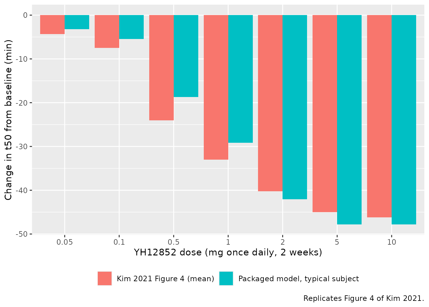
# Deterministic. The shortening grows with dose, and from 0.05 to 2 mg the
# typical subject's value is within 35 % of the published mean. At 5 and
# 10 mg both curves sit on the 45-min floor of the interpolation.
stopifnot(
  all(diff(fig4$dt50_simulated) <= 0),
  all(abs(fig4$dt50_simulated[1:5] / fig4$dt50_published[1:5] - 1) < 0.35),
  all(abs(fig4$dt50_simulated[6:7] - fig4$dt50_published[6:7]) < 5)
)
The typical subject is 12-28 % below the published mean from 0.05 to 1 mg. This is expected: Figure 4 is a mean over virtual subjects, and SLP has large log-normal variability (110.5 %). The mean of a log-normal slope is well above its typical value, so the typical subject understates the mean effect. Kim 2021 also restricted the virtual subjects to parameters inside the 95 % confidence intervals of Table 1 (Methods, PK-PD simulation). That rule cannot be reproduced exactly. At 5 and 10 mg the published decreases level off at about 45-46 min. The same plateau appears here because t50 cannot be read below the first breath sample at 45 min.
Virtual cohorts
The observed data are not public. Two virtual cohorts approximate the trial:
- PK cohort. 100 subjects per dose for the seven tested doses (0.05-3 mg), with weight drawn as in the MD cohort. The rich sampling on Days 1 and 14 follows the Methods.
- GEBT cohort. 200 subjects each at 0.05 and 0.1 mg, drawn like the MLD cohort (weight 58.2 +/- 8.1 kg, 78.6 % women, BMI 21.6 +/- 2.1 kg/m^2). Baseline t10 is log-normal with the Table 2 mean and SD, truncated to the observed 11.1-59.4 min range. The baseline test meal is taken the day before the first dose. The Day-7 test meal is finished at the time of the Day-7 dose.
Occasion 1 is Day 1 and occasion 2 is every later day.
set.seed(20210812)
rxode2::rxSetSeed(20210812)

# Truncated draws by inverse CDF, so that values outside the observed range are
# redrawn rather than piled up at the limits.
rtrunc_norm <- function(n, mean, sd, lo, hi) {
  qnorm(runif(n, pnorm(lo, mean, sd), pnorm(hi, mean, sd)), mean, sd)
}
rtrunc_lnorm <- function(n, meanlog, sdlog, lo, hi) {
  qlnorm(
    runif(n, plnorm(lo, meanlog, sdlog), plnorm(hi, meanlog, sdlog)),
    meanlog, sdlog
  )
}

# PK sampling times after a dose (h), Methods: Day 1 and Day 14 profiles,
# extra Day-14 samples to 72 h, predose troughs on Days 5, 10, 12 and 13.
pk_obs_times <- sort(unique(c(
  c(0, 1, 2, 3, 4, 5, 6, 8, 10, 12, 14, 24),
  13 * 24 + c(0, 1, 2, 3, 4, 5, 6, 8, 10, 12, 14, 24, 36, 48, 72),
  24 * c(4, 9, 11, 12)
)))

make_pk_cohort <- function(n, dose, id_offset) {
  subj <- tibble::tibble(
    id = id_offset + seq_len(n),
    WT = rtrunc_norm(n, 60.4, 8.2, 45.9, 78.8),
    GE_T10_BL = 30,
    treatment = paste(dose, "mg")
  )
  doses <- tidyr::expand_grid(subj, time = seq(0, 13 * 24, by = 24)) |>
    dplyr::mutate(amt = dose, cmt = "depot", evid = 1L, dvid = NA_integer_)
  obs <- tidyr::expand_grid(subj, time = pk_obs_times) |>
    dplyr::mutate(amt = 0, cmt = NA_character_, evid = 0L, dvid = 1L)
  dplyr::bind_rows(doses, obs) |>
    dplyr::mutate(OCC = ifelse(time < 24, 1L, 2L)) |>
    dplyr::arrange(id, time, dplyr::desc(evid))
}

pk_doses <- c(0.05, 0.1, 0.3, 0.5, 1, 2, 3)
pk_events <- dplyr::bind_rows(lapply(seq_along(pk_doses), function(i) {
  make_pk_cohort(100, pk_doses[i], id_offset = (i - 1L) * 100L)
}))
stopifnot(!anyDuplicated(unique(pk_events[, c("id", "time", "evid", "cmt")])))

# GEBT cohort: baseline meal at t = 0, first drug dose at t = 24 h, so Day 7
# of dosing starts at 24 + 6 * 24 = 168 h.
gebt_times <- c(0, 45, 90, 120, 150, 180, 240) / 60
day7_meal <- 24 + 6 * 24
t10_sdlog <- sqrt(log(1 + (15.5 / 30.3)^2))
t10_meanlog <- log(30.3) - t10_sdlog^2 / 2

make_gebt_cohort <- function(n, dose, id_offset) {
  subj <- tibble::tibble(
    id = id_offset + seq_len(n),
    WT = rtrunc_norm(n, 58.2, 8.1, 46.8, 77.3),
    SEXF = rbinom(n, 1, 0.786),
    BMI = rtrunc_norm(n, 21.6, 2.1, 18.2, 25.0),
    GE_T10_BL = rtrunc_lnorm(n, t10_meanlog, t10_sdlog, 11.1, 59.4),
    treatment = paste(dose, "mg")
  )
  doses <- tidyr::expand_grid(subj, time = 24 + seq(0, 13 * 24, by = 24)) |>
    dplyr::mutate(amt = dose, cmt = "depot", evid = 1L, dvid = NA_integer_)
  meals <- tidyr::expand_grid(subj, time = c(0, day7_meal)) |>
    dplyr::mutate(amt = 1e5, cmt = "stomach", evid = 1L, dvid = NA_integer_)
  obs <- tidyr::expand_grid(subj, time = c(gebt_times, day7_meal + gebt_times)) |>
    dplyr::mutate(amt = 0, cmt = NA_character_, evid = 0L, dvid = 1L)
  dplyr::bind_rows(doses, meals, obs) |>
    dplyr::mutate(OCC = ifelse(time < 48, 1L, 2L)) |>
    dplyr::arrange(id, time, dplyr::desc(evid))
}

gebt_events <- dplyr::bind_rows(
  make_gebt_cohort(200, 0.05, id_offset = 10000L),
  make_gebt_cohort(200, 0.1, id_offset = 10200L)
)
stopifnot(!anyDuplicated(unique(gebt_events[, c("id", "time", "evid", "cmt")])))
Simulation
sim_pk <- rxode2::rxSolve(
  mod, pk_events,
  keep = c("treatment", "WT"), useLinCmt = FALSE, returnType = "data.frame"
)
sim_gebt <- rxode2::rxSolve(
  mod, gebt_events,
  keep = c("treatment", "SEXF", "BMI", "GE_T10_BL"),
  useLinCmt = FALSE, returnType = "data.frame"
)
Figure 3a-b: YH12852 concentrations on Days 1 and 14
Kim 2021 Figure 3 is a prediction- and variability-corrected VPC pooled over doses. The plot below shows the 5th, 50th and 95th percentiles of the simulated individual concentrations (without residual error) for each dose.
pk_summ <- sim_pk |>
  dplyr::mutate(
    day = ifelse(time < 24, "Day 1", ifelse(time >= 13 * 24, "Day 14", NA)),
    tsld = ifelse(time < 24, time, time - 13 * 24)
  ) |>
  dplyr::filter(!is.na(day)) |>
  dplyr::group_by(day, treatment, tsld) |>
  dplyr::summarise(
    Q05 = quantile(Cc, 0.05), Q50 = median(Cc), Q95 = quantile(Cc, 0.95),
    .groups = "drop"
  ) |>
  dplyr::mutate(treatment = factor(treatment, paste(pk_doses, "mg"))) |>
  # The Day-1 predose value is zero and cannot be drawn on a log axis.
  dplyr::filter(Q05 > 0)

ggplot(pk_summ, aes(tsld, Q50, colour = treatment, fill = treatment)) +
  geom_ribbon(aes(ymin = Q05, ymax = Q95), alpha = 0.12, colour = NA) +
  geom_line() +
  facet_wrap(~day, scales = "free_x") +
  scale_y_log10() +
  labs(
    x = "Time since last dose (h)", y = "YH12852 plasma concentration (pg/mL)",
    colour = "Dose", fill = "Dose",
    caption = "Compare with Figure 3a-b of Kim 2021 (median and 90% interval)."
  )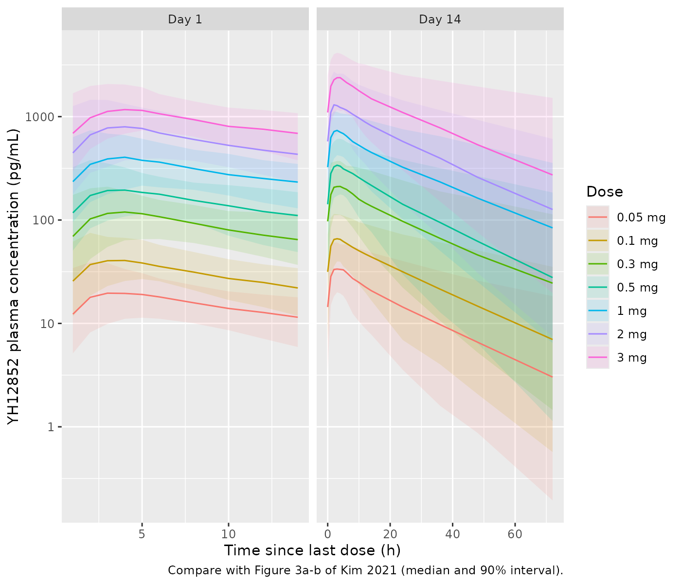
Figure 3c-d and Figure 2: kPCD at baseline and on Day 7
gebt_summ <- sim_gebt |>
  dplyr::mutate(
    visit = ifelse(time < 24, "Baseline", "Day 7"),
    tmeal = ifelse(time < 24, time, time - day7_meal)
  ) |>
  dplyr::group_by(visit, treatment, tmeal) |>
  dplyr::summarise(
    Q05 = quantile(kpcd, 0.05), Q50 = median(kpcd), Q95 = quantile(kpcd, 0.95),
    .groups = "drop"
  )

ggplot(gebt_summ, aes(tmeal, Q50, colour = visit, fill = visit)) +
  geom_ribbon(aes(ymin = Q05, ymax = Q95), alpha = 0.15, colour = NA) +
  geom_line() +
  geom_point() +
  facet_wrap(~treatment) +
  labs(
    x = "Time after completing the test meal (h)", y = "kPCD",
    colour = NULL, fill = NULL,
    caption = "Compare with Figures 2 and 3c-d of Kim 2021 (median and 90% interval)."
  )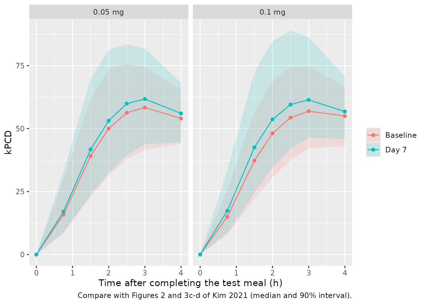
At baseline the median profile rises to a peak of about 60 near 3 h, as in the observed data of Figure 3c. On Day 7 the curve rises earlier and higher, and the spread is wider because SLP is very variable. The paper notes the same overestimated spread in its own VPC.
# Per-subject t50 at baseline and on Day 7, via the Szarka regressions.
t50_subject <- sim_gebt |>
  dplyr::mutate(
    visit = ifelse(time < 24, "baseline", "day7"),
    tmin = round(60 * ifelse(time < 24, time, time - day7_meal))
  ) |>
  dplyr::filter(tmin %in% c(45, 90, 120, 150, 180)) |>
  dplyr::arrange(id, visit, tmin) |>
  dplyr::group_by(id, treatment, visit) |>
  dplyr::summarise(
    t50 = ge_time(szarka_ge(kpcd, SEXF[1], BMI[1]), 0.5),
    .groups = "drop"
  ) |>
  tidyr::pivot_wider(names_from = visit, values_from = t50) |>
  dplyr::mutate(dt50 = day7 - baseline)

t50_tab <- t50_subject |>
  dplyr::group_by(treatment) |>
  dplyr::summarise(
    baseline_t50_mean = mean(baseline, na.rm = TRUE),
    dt50_mean = mean(dt50, na.rm = TRUE),
    dt50_median = median(dt50, na.rm = TRUE),
    .groups = "drop"
  )
t50_tab |>
  dplyr::mutate(dplyr::across(-treatment, \(x) round(x, 1))) |>
  dplyr::rename(
    Dose = treatment,
    "Mean baseline t50 (min)" = baseline_t50_mean,
    "Mean change in t50, Day 7 (min)" = dt50_mean,
    "Median change in t50, Day 7 (min)" = dt50_median
  ) |>
knitr::kable(caption = "Simulated GEBT half time in the MLD-like cohort.")| Dose | Mean baseline t50 (min) | Mean change in t50, Day 7 (min) | Median change in t50, Day 7 (min) |
|---|---|---|---|
| 0.05 mg | 92.1 | -5.5 | -1.7 |
| 0.1 mg | 95.4 | -8.4 | -3.8 |
# Centre-of-distribution gates only, robust to which subjects land in the
# tails. The mean baseline t50 is the Discussion's 94.8 min. Day-7 values are
# checked against the Day-14 bars of Figure 4 (-4.3 and -7.5 min): YH12852
# is near steady state by Day 7. The cohort draws SLP with its full variability
# (unlike the paper's truncated sampling), so the cohort mean may run above
# Figure 4. The bound is loose; the check guards the sign and order of
# magnitude.
stopifnot(
  all(abs(t50_tab$baseline_t50_mean / 94.8 - 1) < 0.15),
  all(t50_tab$dt50_median < 0),
  all(t50_tab$dt50_mean > -30)
)
PKNCA: Day 1 and Day 14
Kim 2021 does not report NCA; the trial’s NCA was published
separately. The check below is that the simulated steady-state
AUC0-24 equals dose / CL, which holds for any
linear model at steady state.
sim_nca <- sim_pk |>
  dplyr::filter(!is.na(Cc)) |>
  dplyr::select(id, time, Cc, treatment)
sim_nca <- dplyr::bind_rows(
  sim_nca,
  sim_nca |> dplyr::distinct(id, treatment) |> dplyr::mutate(time = 0, Cc = 0)
) |>
  dplyr::distinct(id, treatment, time, .keep_all = TRUE) |>
  dplyr::arrange(id, treatment, time)

dose_df <- pk_events |>
  dplyr::filter(evid == 1) |>
  dplyr::select(id, time, amt, treatment)

conc_obj <- PKNCA::PKNCAconc(sim_nca, Cc ~ time | treatment + id)
dose_obj <- PKNCA::PKNCAdose(dose_df, amt ~ time | treatment + id)
intervals <- data.frame(
  start = c(0, 13 * 24),
  end = c(24, 14 * 24),
  cmax = TRUE, tmax = TRUE, auclast = TRUE
)
nca_res <- PKNCA::pk.nca(PKNCA::PKNCAdata(conc_obj, dose_obj, intervals = intervals))

nca_tab <- as.data.frame(nca_res$result) |>
  dplyr::mutate(day = ifelse(start == 0, "Day 1", "Day 14")) |>
  dplyr::group_by(treatment, day, PPTESTCD) |>
  dplyr::summarise(median = median(PPORRES, na.rm = TRUE), .groups = "drop") |>
  tidyr::pivot_wider(names_from = PPTESTCD, values_from = median) |>
  dplyr::mutate(
    dose = as.numeric(sub(" mg", "", treatment)),
    auc_ss_expected = ifelse(day == "Day 14", 1e6 * dose / 88.8, NA)
  ) |>
  dplyr::arrange(dose, day)

nca_tab |>
  dplyr::mutate(dplyr::across(c(cmax, auclast, auc_ss_expected), \(x) signif(x, 3))) |>
  dplyr::select(treatment, day, cmax, tmax, auclast, auc_ss_expected) |>
  dplyr::rename(
    Dose = treatment, Day = day, "Cmax (pg/mL)" = cmax, "Tmax (h)" = tmax,
    "AUC0-24 (pg*h/mL)" = auclast, "dose / CL (pg*h/mL)" = auc_ss_expected
  ) |>
knitr::kable(caption = "Median simulated NCA by dose (100 subjects per dose).")| Dose | Day | Cmax (pg/mL) | Tmax (h) | AUC0-24 (pg*h/mL) | dose / CL (pg*h/mL) |
|---|---|---|---|---|---|
| 0.05 mg | Day 1 | 22.0 | 4.0 | 319 | NA |
| 0.05 mg | Day 14 | 34.6 | 3.0 | 547 | 563 |
| 0.1 mg | Day 1 | 42.3 | 4.0 | 638 | NA |
| 0.1 mg | Day 14 | 68.4 | 3.0 | 1140 | 1130 |
| 0.3 mg | Day 1 | 128.0 | 4.0 | 1820 | NA |
| 0.3 mg | Day 14 | 217.0 | 3.5 | 3600 | 3380 |
| 0.5 mg | Day 1 | 216.0 | 4.0 | 3090 | NA |
| 0.5 mg | Day 14 | 353.0 | 3.0 | 5660 | 5630 |
| 1 mg | Day 1 | 439.0 | 4.0 | 6240 | NA |
| 1 mg | Day 14 | 753.0 | 3.0 | 12300 | 11300 |
| 2 mg | Day 1 | 885.0 | 4.0 | 12000 | NA |
| 2 mg | Day 14 | 1350.0 | 4.0 | 21900 | 22500 |
| 3 mg | Day 1 | 1290.0 | 4.0 | 18800 | NA |
| 3 mg | Day 14 | 2410.0 | 3.0 | 39300 | 33800 |
Assumptions and deviations
-
Omega scale. Table 1 gives every IIV and IOV only
as a percentage. The percentages are read as
100 * sqrt(omega^2), soomega^2 = (pct/100)^2. The supplementary control stream supports this reading. Its initial IOV value on CL, 0.0822, gives exactly the 28.7 % in Table 1 (100 * sqrt(0.0822)= 28.7 %). The alternativelog(1 + CV^2)reading gives 29.3 %. The other initial omegas are too far from their final estimates to discriminate. The choice matters mainly for SLP (110.5 %):omega^2= 1.22 here versus 0.80 under the other reading. -
Unreported covariances. The control stream
estimates the PK etas as a
BLOCK(4)(CL, V2, Q, V3) and the IOV etas as aBLOCK(3). The final covariances are not reported, so the packaged etas are independent. - Body-weight effect on V3, not V2. Table 1 labels the row ‘BWT effect on V2/F’, but the Results text and the control stream both apply it to V3/F. The control stream is followed, with its 59.25 kg reference (the text rounds the median to 59.2 kg).
- Text versus Table 1. The Results prose quotes some IIV and IOV values that differ from Table 1: V3 38.6 %, SLP 116.2 %, IOV CL 28.5 %, V2 48.1 % and Ka 48.9 %. The prose appears to come from an earlier run; Table 1 is used throughout.
-
Residual error on the linear scale. The Methods say
concentrations were log-transformed, but the published control stream
fits
DVwith a combined errorsqrt(prop^2 * IPRED^2 + add^2)on the untransformed scale, with the additive SDs fixed at 0.001. The control stream is followed. -
Control-stream typos. In
$DESthe drug term is defined asEFF1and then used asEFF; Equations 1-2 confirm it isSLP * CONC. THETA(10) is commented ‘COV_AGE exponent’ but multiplies the weight term. -
Units. The control stream computes
CONC = A(2)/V2directly against pg/mL data, so its doses were in ng. The packaged model takes doses in mg and multiplies by 1e6 to giveCcin pg/mL, so SLP keeps its published value (per pg/mL). The pg/mL unit comes from the Figure 3 axis labels and the 30 pg/mL LLOQ. It is also confirmed by the Figure 4 comparison above. A ng/mL reading would make the drug effect about 1000-fold too small to see. - Timing of the GEBT relative to the dose. The test meal was eaten after an overnight fast and the drug was taken after breakfast. The Day-7 (and Day-14) test meal is assumed to be finished at the time of that day’s dose. Figure 3c-d plots kPCD against time since the last dose, which is consistent with this. The baseline GEBT is simulated drug-free, on the day before the first dose.
- Figure 4 cohort. Kim 2021 simulated 150 virtual subjects per dose. It kept only subjects whose PK-PD parameters were inside the Table 1 95 % confidence intervals, and derived BMI from sex and weight with a regression that is not published. That cohort cannot be rebuilt, so Figure 4 is compared with the typical subject. The Figure 4 values were read off the bar chart by the maintainers.
- GEBT t10 distribution. The baseline t10 of the virtual GEBT cohort is log-normal with the Table 2 mean and SD, truncated to the observed range. Table 2 does not give the shape of the distribution.
- Ghoos model not packaged. The alternative empirical Ghoos PK-PD model (Equation 5, Table S2) was not selected as final and is not included.
- No erratum or correction notice was found for Kim 2021 as of 2026-09-28.