Linear monoclonal antibody PK across species (Betts 2018)
Source:vignettes/articles/Betts_2018_mAb_linear_PK.Rmd
Betts_2018_mAb_linear_PK.RmdModel and source
Betts et al. (2018) pooled individual-level IV concentration-time data for 27 Pfizer monoclonal antibodies (mAbs) with linear (non-target-mediated) clearance across three species (human, cynomolgus monkey, and hFcRn Tg32 transgenic mouse). The analysis yields a single set of typical class-level two-compartment popPK parameters per species (Table 2), and a combined jointly-fitted model with bodyweight-based allometric scaling on all four disposition parameters (Table 4).
Four model files are packaged for this paper. Each represents an independent NONMEM fit reported in the source:
-
Betts_2018_mAb_human-Table 2, Human column (n=18 mAbs). -
Betts_2018_mAb_cyno-Table 2, Cynomolgus Monkey column (n=23 mAbs). -
Betts_2018_mAb_tg32mouse-Table 2, Tg32 hFcRn Transgenic Mouse column (n=11 mAbs). -
Betts_2018_mAb_combined-Table 4, all-species combined fit with allometric scaling (n=27 mAbs).
Article: https://doi.org/10.1080/19420862.2018.1462429
mod_human    <- readModelDb("Betts_2018_mAb_human")
mod_cyno     <- readModelDb("Betts_2018_mAb_cyno")
mod_tg32     <- readModelDb("Betts_2018_mAb_tg32mouse")
mod_combined <- readModelDb("Betts_2018_mAb_combined")

cat(mod_human()$description, "\n\n", mod_human()$reference, sep = "")
#> Class-level typical two-compartment population PK model for monoclonal antibodies with linear clearance in adult humans (Betts 2018, n=18 mAbs).
#>
#> Betts A, Keunecke A, van Steeg TJ, van der Graaf PH, Avery LB, Jones H, Berkhout J. Linear pharmacokinetic parameters for monoclonal antibodies are similar within a species and across different pharmacological targets: A comparison between human, cynomolgus monkey and hFcRn Tg32 transgenic mouse using a population-modeling approach. MAbs. 2018;10(5):751-64. doi:10.1080/19420862.2018.1462429
Population
The source dataset pools Pfizer historical individual concentration-time data from 27 mAbs with linear PK. Human data (n=18 mAbs) were from healthy volunteers or patients receiving single-dose IV mAb at 3-24 individuals per dose level. Cynomolgus monkey data (n=23 mAbs) were single-dose IV preclinical PK at 1-3 dose levels with two monkeys per dose. hFcRn Tg32 transgenic mouse data (n=11 mAbs) were single-dose IV at 3.5 mg/kg (1 mAb) or 5 mg/kg (10 mAbs), n=5-6 per mAb. Non-linear (target-mediated) doses were excluded from the fits by combining visual inspection with a linear dose-vs.-AUC deviation test (Betts 2018 Fig. 1). Reference body weights for the assumed preclinical species were 3 kg (cynomolgus monkey) and 0.02 kg (hFcRn Tg32 mouse); human body weights were subject-specific.
Table 1 of the source lists each of the 27 mAbs, its immunoglobulin subclass (12 IgG1, 15 IgG2), its target class (16 soluble, 9 membrane, 2 mixed), and the retained linear dose range per species.
Source trace
The per-parameter origin is recorded as an in-file comment next to
each ini() entry in
inst/modeldb/specificDrugs/Betts_2018_mAb_*.R. The
consolidated table below spans all four packaged models.
| Model | Parameter | Value (paper units) | Absolute value used | Source location |
|---|---|---|---|---|
| Human | CL | 0.15 mL/h/kg | 0.252 L/day (70 kg) | Table 2, Human column |
| Human | V1 | 46.31 mL/kg | 3.2417 L (70 kg) | Table 2, Human column |
| Human | Q | 0.27 mL/h/kg | 0.4536 L/day (70 kg) | Table 2, Human column |
| Human | V2 | 31.47 mL/kg | 2.2029 L (70 kg) | Table 2, Human column |
| Human | IIV CL / cov / V1 | 0.48 / 0.09 / 0.09 | (log-scale variances) | Table 2, Human column |
| Cynomolgus monkey | CL | 0.27 mL/h/kg | 0.01944 L/day (3 kg) | Table 2, Cynomolgus column |
| Cynomolgus monkey | V1 | 39.29 mL/kg | 0.11787 L (3 kg) | Table 2, Cynomolgus column |
| Cynomolgus monkey | Q | 1.00 mL/h/kg | 0.072 L/day (3 kg) | Table 2, Cynomolgus column |
| Cynomolgus monkey | V2 | 27.56 mL/kg | 0.08268 L (3 kg) | Table 2, Cynomolgus column |
| Cynomolgus monkey | IIV CL / cov / V1 | 0.38 / 0.09 / 0.10 | (log-scale variances) | Table 2, Cynomolgus column |
| hFcRn Tg32 mouse | CL | 0.35 mL/h/kg | 0.000168 L/day (0.02 kg) | Table 2, Tg32 Mouse column |
| hFcRn Tg32 mouse | V1 | 59.28 mL/kg | 0.0011856 L (0.02 kg) | Table 2, Tg32 Mouse column |
| hFcRn Tg32 mouse | Q | 4.40 mL/h/kg | 0.002112 L/day (0.02 kg) | Table 2, Tg32 Mouse column |
| hFcRn Tg32 mouse | V2 | 60.54 mL/kg | 0.0012108 L (0.02 kg) | Table 2, Tg32 Mouse column |
| hFcRn Tg32 mouse | IIV CL / cov / V1 | 0.41 / 0.11 / 0.12 | (log-scale variances) | Table 2, Tg32 Mouse column |
| Combined (all species) | CL | 0.16 mL/h/kg | 0.2688 L/day (70 kg ref) | Table 4, all-species column |
| Combined (all species) | V1 | 45.19 mL/kg | 3.1633 L (70 kg ref) | Table 4, all-species column |
| Combined (all species) | Q | 0.28 mL/h/kg | 0.4704 L/day (70 kg ref) | Table 4, all-species column |
| Combined (all species) | V2 | 30.81 mL/kg | 2.1567 L (70 kg ref) | Table 4, all-species column |
| Combined (all species) | alpha (CL) | 0.89 | 0.89 | Table 4, all-species column |
| Combined (all species) | beta (V1) | 0.98 | 0.98 | Table 4, all-species column |
| Combined (all species) | gamma (Q) | 0.67 | 0.67 | Table 4, all-species column |
| Combined (all species) | delta (V2) | 0.95 | 0.95 | Table 4, all-species column |
| Combined (all species) | IIV CL / cov / V1 | 0.47 / 0.08 / 0.11 | (log-scale variances) | Table 4, all-species column |
| All models | 2-cpt IV disposition | - | - | Fig. 1a and Materials and methods “PK model” |
| All models | Proportional error per cpd | - | fixed(0) per policy | Table 2 / Table 4 footnote, per-compound values in Supp. Table 1 / 2 (not available) |
All weight-normalized values were converted to absolute units at the species-representative body weight used in the source fit (70 kg human, 3 kg cynomolgus monkey, 0.02 kg hFcRn Tg32 mouse) and to days for tractability of the mAb ~2-4 week terminal half-life.
Virtual cohort -human single-dose 1 mg/kg IV
The Betts 2018 popPK model is a class-level “typical” 2-compartment IV model. To reproduce the source Fig. 4 concentration-vs-time envelope, we simulate a virtual cohort of 200 typical adults each receiving a single 1 mg/kg IV dose (70 kg reference body weight), followed for 42 days.
set.seed(29634430L)

sim_time_days <- 42
grid_days     <- c(0, 0.25, 0.5, 1, 2, 3, 5, 7, 10, 14, 21, 28, 35, 42)

n_human <- 200
events_human <- dplyr::bind_rows(
  tibble::tibble(
    id   = seq_len(n_human),
    time = 0,
    amt  = 70,           # 1 mg/kg * 70 kg
    evid = 1,
    cmt  = "central"
  ),
  tidyr::expand_grid(
    id   = seq_len(n_human),
    time = grid_days
  ) |>
    dplyr::mutate(amt = NA_real_, evid = 0, cmt = "central")
) |>
  dplyr::arrange(id, time, dplyr::desc(evid))
Human simulation
sim_human <- rxode2::rxSolve(mod_human, events = events_human) |>
  as.data.frame() |>
  dplyr::mutate(species = "Human (70 kg, 1 mg/kg IV)")
Replicating Fig. 4 -dose-normalized concentration envelope
Fig. 4 of Betts 2018 shows the median plus 5th and 95th percentiles of 200 bootstrap samples of the combined-species PK model, plotted as dose-normalized concentration (ng/mL) vs time (hours). Here we render the same envelope for the human single-species model, keeping the same concentration axis by expressing the simulated Cc per mg dose and converting from mg/L to ng/mL (multiplying by 1000).
env_human <- sim_human |>
  dplyr::group_by(time) |>
  dplyr::summarise(
    Q05 = quantile(Cc, 0.05, na.rm = TRUE),
    Q50 = quantile(Cc, 0.50, na.rm = TRUE),
    Q95 = quantile(Cc, 0.95, na.rm = TRUE),
    .groups = "drop"
  ) |>
  dplyr::mutate(
    time_h = time * 24,
    Q05_ngml_per_mg = Q05 / 70 * 1000,
    Q50_ngml_per_mg = Q50 / 70 * 1000,
    Q95_ngml_per_mg = Q95 / 70 * 1000
  ) |>
  dplyr::filter(time > 0)

ggplot(env_human, aes(time_h, Q50_ngml_per_mg)) +
  geom_ribbon(aes(ymin = Q05_ngml_per_mg, ymax = Q95_ngml_per_mg),
              alpha = 0.2, fill = "steelblue") +
  geom_line(colour = "steelblue", linewidth = 0.8) +
  scale_x_continuous(name = "Time (hours)") +
  scale_y_log10(name = "Dose-normalized Cc (ng/mL per mg)") +
  labs(title = "Replicates Fig. 4 shape for the human single-species model",
       caption = "Median and 5-95% percentile of Cc for 200 virtual humans after 1 mg/kg IV.") +
  theme_minimal()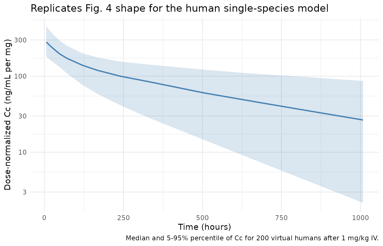
Cross-species simulation
We simulate 100 virtual subjects per preclinical species at their species-typical single IV dose and plot the typical concentration-time profiles (no residual noise) on the same absolute time axis, in units of dose-normalized Cc.
n_pre  <- 100
grid_h <- c(0, 6, 12, 24, 48, 72, 96, 168, 240, 336, 504, 672, 1008) / 24  # hours -> days

make_events <- function(n, dose_mg, id_offset = 0L) {
  dplyr::bind_rows(
    tibble::tibble(id = id_offset + seq_len(n), time = 0, amt = dose_mg,
                   evid = 1, cmt = "central"),
    tidyr::expand_grid(id = id_offset + seq_len(n), time = grid_h) |>
      dplyr::mutate(amt = NA_real_, evid = 0, cmt = "central")
  ) |> dplyr::arrange(id, time, dplyr::desc(evid))
}

events_cyno <- make_events(n_pre, dose_mg = 3,     id_offset =    0L) # 1 mg/kg * 3 kg
events_tg32 <- make_events(n_pre, dose_mg = 0.10,  id_offset = 1000L) # 5 mg/kg * 0.02 kg

sim_cyno <- rxode2::rxSolve(mod_cyno, events = events_cyno) |>
  as.data.frame() |>
  dplyr::mutate(species = "Cyno (3 kg, 1 mg/kg IV)",
                dose_mg = 3)

sim_tg32 <- rxode2::rxSolve(mod_tg32, events = events_tg32) |>
  as.data.frame() |>
  dplyr::mutate(species = "Tg32 mouse (0.02 kg, 5 mg/kg IV)",
                dose_mg = 0.10)

sim_human_h <- sim_human |>
  dplyr::mutate(dose_mg = 70)

cross <- dplyr::bind_rows(
  sim_human_h |> dplyr::select(id, time, Cc, species, dose_mg),
  sim_cyno    |> dplyr::select(id, time, Cc, species, dose_mg),
  sim_tg32    |> dplyr::select(id, time, Cc, species, dose_mg)
) |>
  dplyr::group_by(species, time) |>
  dplyr::summarise(
    Q05 = quantile(Cc / dose_mg[1] * 1000, 0.05, na.rm = TRUE),
    Q50 = quantile(Cc / dose_mg[1] * 1000, 0.50, na.rm = TRUE),
    Q95 = quantile(Cc / dose_mg[1] * 1000, 0.95, na.rm = TRUE),
    .groups = "drop"
  ) |>
  dplyr::filter(time > 0)

ggplot(cross, aes(time, Q50, colour = species, fill = species)) +
  geom_ribbon(aes(ymin = Q05, ymax = Q95), alpha = 0.15, colour = NA) +
  geom_line(linewidth = 0.7) +
  scale_x_continuous(name = "Time (days)") +
  scale_y_log10(name = "Dose-normalized Cc (ng/mL per mg)") +
  labs(title = "Species comparison -dose-normalized Cc from the single-species popPK fits",
       caption = "Median and 5-95% percentile per species.") +
  theme_minimal() +
  theme(legend.position = "bottom")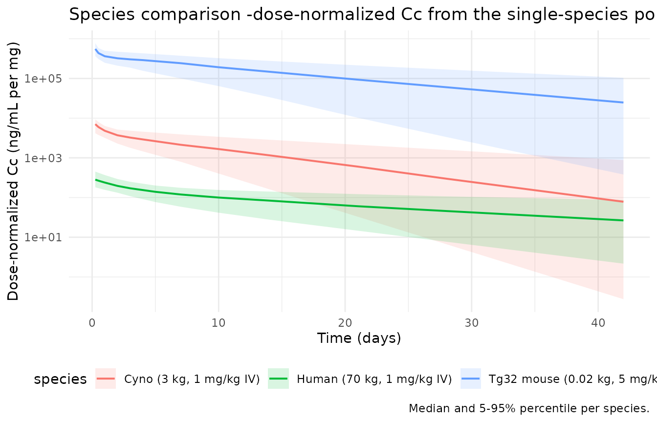
Consistent with Betts 2018 Fig. 2 and 3: mouse concentration falls fastest (highest weight-normalized CL, smallest volume), then cyno, then human; volumes of distribution approximate species plasma volume (30-60 mL/kg).
Combined-species allometric model demonstration
The combined-species model in Table 4 is a single joint fit of all 27 mAbs across all three species using estimated bodyweight allometric exponents on CL (0.89), V1 (0.98), Q (0.67), and V2 (0.95) with reference 70 kg. We compare the typical predictions from the combined-species model at species-representative body weights (70 kg, 3 kg, 0.02 kg) against the single-species fits above.
mod_combined_typical <- mod_combined |> rxode2::zeroRe()

grid_combined <- c(0, 0.25, 0.5, 1, 2, 3, 5, 7, 10, 14, 21, 28, 35, 42)

events_combined <- dplyr::bind_rows(
  tibble::tibble(id = 1L, time = 0, amt = 70,    evid = 1, cmt = "central", WT = 70),
  tibble::tibble(id = 2L, time = 0, amt = 3,     evid = 1, cmt = "central", WT = 3),
  tibble::tibble(id = 3L, time = 0, amt = 0.10,  evid = 1, cmt = "central", WT = 0.02),
  tidyr::expand_grid(
    id   = c(1L, 2L, 3L),
    time = grid_combined
  ) |>
    dplyr::mutate(amt = NA_real_, evid = 0, cmt = "central",
                  WT = dplyr::case_when(id == 1L ~ 70,
                                        id == 2L ~ 3,
                                        id == 3L ~ 0.02))
) |>
  dplyr::arrange(id, time, dplyr::desc(evid))

sim_combined <- rxode2::rxSolve(mod_combined_typical,
                                events = events_combined,
                                keep = c("WT")) |>
  as.data.frame() |>
  dplyr::mutate(
    species = dplyr::case_when(
      id == 1L ~ "Human (70 kg)",
      id == 2L ~ "Cyno (3 kg)",
      id == 3L ~ "Tg32 mouse (0.02 kg)"
    ),
    dose_mg = dplyr::case_when(
      id == 1L ~ 70,
      id == 2L ~ 3,
      id == 3L ~ 0.10
    ),
    Cc_ngml_per_mg = Cc / dose_mg * 1000
  )
#> ℹ omega/sigma items treated as zero: 'etalcl', 'etalvc'
#> Warning: multi-subject simulation without without 'omega'

ggplot(sim_combined |> dplyr::filter(time > 0),
       aes(time, Cc_ngml_per_mg, colour = species)) +
  geom_line(linewidth = 0.8) +
  scale_x_continuous(name = "Time (days)") +
  scale_y_log10(name = "Dose-normalized Cc (ng/mL per mg)") +
  labs(title = "Combined-species allometric model -typical predictions per species",
       caption = "Typical (zero-eta) predictions from the Betts 2018 Table 4 all-species combined fit.") +
  theme_minimal() +
  theme(legend.position = "bottom")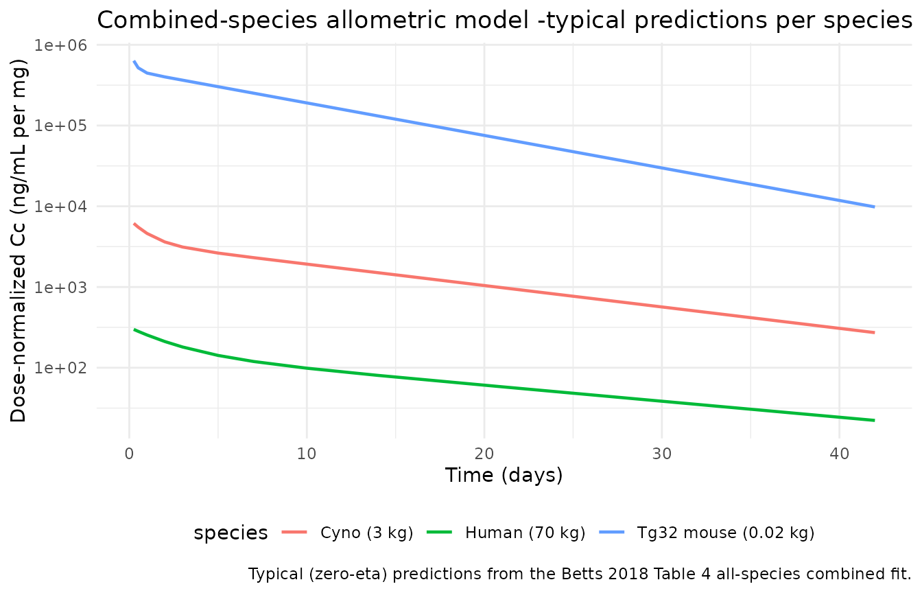
PKNCA validation
We run PKNCA on the human single-species simulation to derive Cmax, Tmax, AUC0-inf, and terminal t1/2 per subject, then summarize the median and IQR across the 200-subject cohort. All computed values are for a single 1 mg/kg IV dose (dose_mg = 70) in a typical 70 kg adult.
sim_nca <- sim_human |>
  dplyr::filter(!is.na(Cc)) |>
  dplyr::select(id, time, Cc) |>
  dplyr::mutate(treatment = "1 mg/kg IV")

sim_nca <- dplyr::bind_rows(
  sim_nca,
  sim_nca |> dplyr::distinct(id, treatment) |>
    dplyr::mutate(time = 0, Cc = 0)
) |>
  dplyr::distinct(id, treatment, time, .keep_all = TRUE) |>
  dplyr::arrange(id, treatment, time)

conc_obj <- suppressMessages(
  PKNCA::PKNCAconc(sim_nca, Cc ~ time | treatment + id)
)

dose_df <- events_human |>
  dplyr::filter(evid == 1) |>
  dplyr::mutate(treatment = "1 mg/kg IV") |>
  dplyr::select(id, time, amt, treatment)

dose_obj <- suppressMessages(
  PKNCA::PKNCAdose(dose_df, amt ~ time | treatment + id)
)

intervals <- data.frame(
  start       = 0,
  end         = Inf,
  cmax        = TRUE,
  tmax        = TRUE,
  aucinf.obs  = TRUE,
  half.life   = TRUE
)

nca_data <- suppressMessages(
  PKNCA::PKNCAdata(conc_obj, dose_obj, intervals = intervals)
)
nca_res  <- suppressMessages(suppressWarnings(PKNCA::pk.nca(nca_data)))

nca_summary <- as.data.frame(nca_res$result) |>
  dplyr::filter(PPTESTCD %in% c("cmax", "tmax", "aucinf.obs", "half.life")) |>
  dplyr::group_by(PPTESTCD) |>
  dplyr::summarise(
    median = median(PPORRES, na.rm = TRUE),
    p05    = quantile(PPORRES, 0.05, na.rm = TRUE),
    p95    = quantile(PPORRES, 0.95, na.rm = TRUE),
    .groups = "drop"
  )

nca_summary |>
  dplyr::rename(`NCA parameter` = PPTESTCD,
                `Median` = median,
                `5th percentile` = p05,
                `95th percentile` = p95) |>
  knitr::kable(digits = 3,
caption = "PKNCA-derived Cmax (mg/L), Tmax (day), AUC0-inf (mg*day/L), and terminal t1/2 (day) across the 200-subject virtual human cohort after 1 mg/kg IV.")| NCA parameter | Median | 5th percentile | 95th percentile |
|---|---|---|---|
| aucinf.obs | 281.555 | 104.321 | 763.554 |
| cmax | 20.972 | 13.196 | 34.181 |
| half.life | 16.692 | 7.613 | 43.189 |
| tmax | 0.000 | 0.000 | 0.000 |
Consistency with paper’s reported literature comparators
Betts 2018 Table 3 lists CL, V1, Q, V2 for five clinical mAbs with
linear PK (bevacizumab, infliximab, pertuzumab, rituximab, trastuzumab)
alongside the human popPK estimates from this study. The comparison
below shows the paper’s own reported values, converted to absolute units
for a 70 kg adult, next to the Betts 2018 Human popPK typical-value
column that this vignette’s Betts_2018_mAb_human model
encodes. This is a fidelity check on the encoding rather than an
external validation -the observed similarity between the five clinical
mAbs and the Betts 2018 human popPK typical values is a headline result
of the paper (Table 3).
tab3 <- tibble::tribble(
  ~mAb,                     ~cl_mLhkg, ~vc_mLkg, ~q_mLhkg, ~vp_mLkg,
  "Betts 2018 Human popPK", 0.15,      46.31,    0.27,     31.47,
  "Bevacizumab",            0.12,      38.0,     0.35,     39.4,
  "Infliximab (AS)",        0.16,      43.7,     1.02,     42.0,
  "Infliximab (UC)",        0.24,      47.0,     4.25,     59.0,
  "Pertuzumab",             0.13,      39.1,     0.33,     30.9,
  "Rituximab",              0.15,      42.6,     0.39,     52.0,
  "Trastuzumab",            0.13,      42.1,     0.29,     68.4
)

tab3 |>
  dplyr::rename(
    "mAb"           = mAb,
    "CL (mL/h/kg)"  = cl_mLhkg,
    "V1 (mL/kg)"    = vc_mLkg,
    "Q (mL/h/kg)"   = q_mLhkg,
    "V2 (mL/kg)"    = vp_mLkg
  ) |>
knitr::kable(caption = "Betts 2018 Table 3: Human popPK typical values vs five literature comparator clinical mAbs.")| mAb | CL (mL/h/kg) | V1 (mL/kg) | Q (mL/h/kg) | V2 (mL/kg) |
|---|---|---|---|---|
| Betts 2018 Human popPK | 0.15 | 46.31 | 0.27 | 31.47 |
| Bevacizumab | 0.12 | 38.00 | 0.35 | 39.40 |
| Infliximab (AS) | 0.16 | 43.70 | 1.02 | 42.00 |
| Infliximab (UC) | 0.24 | 47.00 | 4.25 | 59.00 |
| Pertuzumab | 0.13 | 39.10 | 0.33 | 30.90 |
| Rituximab | 0.15 | 42.60 | 0.39 | 52.00 |
| Trastuzumab | 0.13 | 42.10 | 0.29 | 68.40 |
Infliximab for ulcerative colitis is an outlier (CL 0.24 mL/h/kg, Q 4.25 mL/h/kg) as noted in Betts 2018; the other four literature comparators sit inside the reported 95% CIs of the class-level human popPK estimates.
Assumptions and deviations
- Class-level, not compound-specific. All four packaged models represent the pooled typical class-level PK across many mAbs (18, 23, 11, and 27 respectively). They are intended for early-stage popPK simulation, cross-species prediction, and initial-value seeding for compound-specific fits -not for reproducing any single named mAb’s PK profile. Per-compound residual errors were reported per-compound in the Betts 2018 Supplementary Tables 1 and 2.
-
Residual error fixed at 0. The paper’s Table 2 and
Table 4 footnotes state “Residual errors per compound are shown in
Supplementary Table 1” (or 2); the supplement was not available when
this model was built, so no class-level typical proportional residual
value could be sourced. Per the package’s standing policy for unreported
RUV,
propSdis wrapped infixed(0)in every packaged model. Users needing residual noise for simulation should override with a domain-appropriate typical value (mAb popPK residuals are commonly 15-25% CV) or supply the compound-specific value from the supplement when acquired. -
Reference body weights. The single-species
preclinical models (
Betts_2018_mAb_cyno,Betts_2018_mAb_tg32mouse) fix the absolute parameters at the species-representative body weights the paper’s Materials and methods declared (3 kg and 0.02 kg respectively). Real subjects are unlikely to sit exactly at those weights; the combined- species model (Betts_2018_mAb_combined) is the appropriate choice when species-specific body weight varies materially across the simulated cohort, via its allometric exponents on all four disposition parameters. -
Absolute unit conversion. Betts 2018 reports
parameters in weight-normalized units (mL/h/kg for CL and Q, mL/kg for
V1 and V2, per hour of time). All packaged models express parameters in
absolute units (L for volumes, L/day for clearances) -day units align
with typical mAb elimination timescales, and absolute-unit rxode2 event
tables need no weight-normalization guard-rails per subject. The
arithmetic conversions are recorded in-line in every model file’s
ini()block. - Body-weight ranges outside published support. The combined-species allometric model’s exponents (Table 4) were fit on data spanning 0.02-70 kg. Simulating outside this range (e.g. rat or dog body weights in the interior, or elephant / whale body weights beyond it) is extrapolation and not validated against the source data.
-
Excluded from packaging. The two intermediate
combined-dataset fits (Cyno + Human column of Table 4, and Tg32 Mouse +
Human column of Table 4) are structural duplicates of
Betts_2018_mAb_combinedwith only the fitted dataset differing. Their function is illustrative (comparing the allometric exponents that a single preclinical species yields against the all-species fit) rather than distinct simulation targets, so they are not shipped as separate model files. Their exponents are listed in Betts 2018 Table 4 for readers who need them.