Hydroxyurea (Pandey 2023)
Source:vignettes/articles/Pandey_2023_hydroxyurea.Rmd
Pandey_2023_hydroxyurea.RmdModel and source
- Citation: Pandey A, Raja R, Estepp JH, Ramkrishna D (2023). Leveraging mathematical modeling to analyze nonadherence for hydroxyurea therapy in sickle cell disease. CPT Pharmacometrics Syst Pharmacol 12(6):748-758. doi:10.1002/psp4.12945. Model equations and parameter values from the parent paper: Pandey A, Estepp JH, Raja R, Kang G, Ramkrishna D (2022). Mathematical modeling of hydroxyurea therapy in individuals with sickle cell disease. Pharmaceutics 14(5):1065. doi:10.3390/pharmaceutics14051065.
- Description: Semi-mechanistic PK-PD model of oral hydroxyurea in children with sickle cell disease (HUSTLE trial, NCT00305175), used by Pandey 2023 to study treatment nonadherence. PK: Savic transit-compartment absorption (Nt + 1 compartments, rate ktr) into a plasma compartment with first-order elimination ke; plasma volume from the Nadler blood-volume equation (or 70 mL/kg below 25 kg) times (1 - HCT/100). The pharmacodynamic driver is the daily average plasma concentration (piecewise constant within each dosing day, zero on a missed day). Erythropoiesis: stem-cell pool with Hill feedback from circulating red cells, three maturation compartments, and circulating red cells; hydroxyurea kills stem cells and prolongs red-cell lifespan (saturable). Mean cell volume (MCV) rises linearly with the daily average concentration. Mean cell fetal hemoglobin (HbF, pg) is induced through a Michaelis-Menten-formed intermediate acting via a Hill function. The model was fitted subject by subject (no population variability or residual error); typical values are the HUSTLE cohort central values of the parent paper (Pandey 2022).
- Article: https://doi.org/10.1002/psp4.12945 (open access; Appendix S1 holds the model equations, Text S2, and the per-participant estimates, Tables S1-S4)
- Parent model paper: https://doi.org/10.3390/pharmaceutics14051065 (Pandey 2022, open access; PK estimates in Table 2, cohort summaries of the pharmacodynamic estimates in Tables 3 and 5)
Pandey 2023 studies how missed hydroxyurea doses change two biomarkers of response in sickle cell disease, mean cell volume (MCV) and fetal hemoglobin (HbF). It reuses the integrated PK-PD model of Pandey 2022, which it reprints in Text S2. Hydroxyurea is absorbed through a transit chain and eliminated first-order; the daily average plasma concentration drives (i) a five-pool erythropoiesis model in which the drug kills stem cells and lengthens red-cell lifespan, (ii) a mean-cell-volume balance in which new cells are larger in proportion to the concentration, and (iii) a two-step HbF induction model. The authors fitted every participant separately by weighted least squares, so the model has no between-subject variability or residual error. The packaged typical values are the HUSTLE cohort central values printed in Pandey 2022; the 2023 per-participant estimates are reproduced further below.
Population
Pandey 2023 analysed 40 children and adolescents with sickle cell disease from the HUSTLE trial (NCT00305175, St. Jude Children’s Research Hospital) whose MCV or HbF fell during treatment in a way their pharmacy refill records did not explain. Participants receiving transfusions, with sparse or gapped data, or whose biomarkers were already explained by the refill records were excluded. The paper does not tabulate demographics for the 40. The parent analysis of 85 HUSTLE participants (Pandey 2022 Table 1) reports a starting age of 10.12 (SD 4.72) years, 54 male / 31 female, and baseline MCV 85.34 fL, MCH 29.76 pg, HbF 8.0%, hematocrit 23.46% and red-cell count 2.777 x 10^6 cells/uL.
str(rxode2::rxode(readModelDb("Pandey_2023_hydroxyurea"))$population)
#> List of 10
#>  $ species       : chr "human"
#>  $ n_subjects    : int 40
#>  $ n_studies     : int 1
#>  $ age_range     : chr "children and adolescents; HUSTLE cohort starting age 10.12 (SD 4.72) years (Pandey 2022 Table 1)"
#>  $ sex_female_pct: num 36.5
#>  $ race_ethnicity: chr "not reported"
#>  $ disease_state : chr "Sickle cell disease on daily oral hydroxyurea (HUSTLE, NCT00305175, St. Jude Children's Research Hospital). The"| __truncated__
#>  $ dose_range    : chr "Daily oral dose computed per visit interval from pharmacy refill records (Pandey 2023 Text S1)"
#>  $ regions       : chr "United States (Memphis, TN)"
#>  $ notes         : chr "The parent analysis (Pandey 2022) fitted the same equations to 85 HUSTLE participants (54 male / 31 female; Tab"| __truncated__
Source trace
| Equation / parameter | Value | Source location |
|---|---|---|
Transit input F D ktr (ktr t)^Nt exp(-ktr t) / Nt! into
plasma |
n/a | Pandey 2023 Text S2 Eqs. S.2-S.3; Pandey 2022 Eq. 1 |
Vp = Vb (1 - HCT/100); Nadler Vb (WT >=
25 kg) or 70 mL/kg |
n/a | Pandey 2023 Text S2 Eqs. S.4-S.6; Pandey 2022 Eqs. 2-4 |
| Daily average concentration drives the PD | n/a | Pandey 2023 Text S2, last paragraph of the PK section |
Erythropoiesis ODEs, Hill feedback, kdse(Cp),
kde(Cp)
|
n/a | Pandey 2023 Text S2 Eqs. S.7-S.10 |
kpe,max = kte Nse(0) (Psi^g + Ne(0)^g) / Psi^g |
n/a | Pandey 2023 Tables S1-S2 footnote |
| MCV ODE | n/a | Pandey 2023 Text S2 Eq. S.12 |
HbF intermediate and mean cell HbF ODEs;
kbf = kdf Fm(0)
|
n/a | Pandey 2023 Text S2 Eqs. S.13-S.14; Tables S3-S4 footnote |
Fm = HbF(%) / 100 x MCH |
n/a | Pandey 2023 Text S2 Eq. S.1 |
F |
0.12 | Pandey 2022 Table 2 (mean) |
ktr |
5.02 1/h | Pandey 2022 Table 2 (mean) |
Nt |
1.14 | Pandey 2022 Table 2 (mean) |
ke |
0.54 1/h | Pandey 2022 Table 2 (mean) |
Psi_e |
2.2 x 10^11 cells/L | Pandey 2022 Table 3 (median) |
gamma_e |
1.6 | Pandey 2022 Table 3 (median) |
kdse,max |
0.17 1/day | Pandey 2022 Table 3 (median) |
Kdse,50 |
0.43 uM | Pandey 2022 Table 3 (median) |
kte |
0.2 1/day | Pandey 2022 Table 3 (median) |
kde,max |
0.03 1/day | Pandey 2022 Table 3 (median) |
Kde,50 |
310 uM | Pandey 2022 Table 3 (median) |
alpha |
0.37 fL/uM | Pandey 2022 Table 3 (median) |
kmet |
1.2 uM/day | Pandey 2022 Table 5 (median) |
Kmet |
27 uM | Pandey 2022 Table 5 (median) |
kdi |
0.03 1/day | Pandey 2022 Table 5 (median) |
kaf |
1.5 pg/day | Pandey 2022 Table 5 (median) |
Kaf |
13 uM | Pandey 2022 Table 5 (median) |
n |
3.2 | Pandey 2022 Table 5 (median) |
kdf |
0.07 1/day | Pandey 2022 Table 5 (median) |
Baseline red-cell count Ne(0)
|
2.777 x 10^12 cells/L | Pandey 2022 Table 1 (baseline mean) |
Baseline MCV Vm0
|
85.34 fL | Pandey 2022 Table 1 (baseline mean) |
Baseline mean cell HbF Fm(0)
|
8.004% x 29.76 pg = 2.38 pg | Pandey 2022 Table 1 (baseline means) with Eq. S.1 |
Typical participant and dosing
The figures below use one typical participant: a 30 kg, 135 cm boy with the HUSTLE baseline hematocrit of 23.46%, taking 20 mg/kg (600 mg) once a day. Pandey 2023 does not report the covariates, baselines or dose history of the representative participant in its Figures 4-6, so the figures are reproduced in shape rather than value.
mod <- readModelDb("Pandey_2023_hydroxyurea")
ui <- rxode2::rxode(mod)
covs <- data.frame(WT = 30, HT = 135, SEXF = 0, HCT = 23.46)
dose_mg <- 20 * covs$WT

# Build a dosing history from the days on which a dose is taken, with a
# daily observation grid. Doses sort before observations at the same time,
# so the observation at day d carries day d's average concentration.
make_regimen <- function(id, label, dose_days, n_days) {
  doses <- data.frame(
    id = rep(id, length(dose_days)), time = dose_days, evid = rep(1L, length(dose_days)),
    amt = rep(dose_mg, length(dose_days)), cmt = rep("depot", length(dose_days))
  )
  obs <- data.frame(id = id, time = seq(0, n_days), evid = 0L, amt = 0, cmt = "central")
  dplyr::bind_rows(doses, obs) |>
    dplyr::mutate(regimen = label) |>
    dplyr::arrange(time, dplyr::desc(evid)) |>
    cbind(covs)
}
# A step cap below one day keeps LSODA from stepping across a day's sharp
# absorption peak on these multi-year daily-dosing courses; without it the
# solver can exhaust its step budget.
solve_days <- function(events, ...) {
  events <- dplyr::arrange(events, id, time, dplyr::desc(evid))
  sim <- rxode2::rxSolve(mod, events = events, keep = "regimen", maxsteps = 1e6, hmax = 0.1, ...) |>
    as.data.frame()
  if (is.null(sim$id)) sim$id <- events$id[1]
  sim |> dplyr::filter(time == round(time))
}
Pharmacokinetics
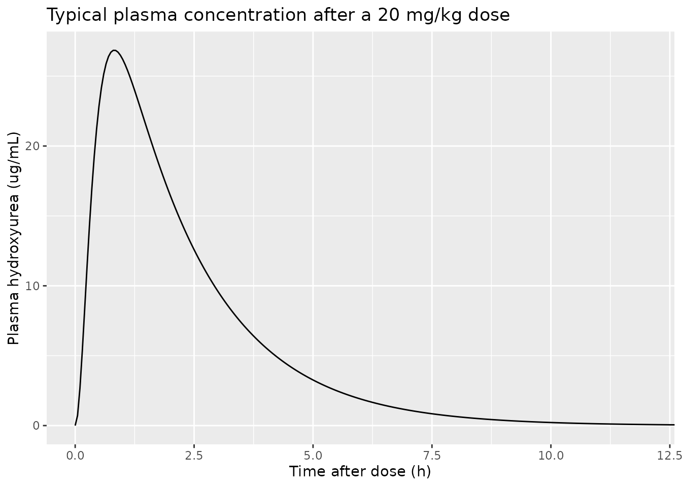
A single 20 mg/kg dose, the dose at which HUSTLE collected its PK profiles (the PK estimates of Pandey 2022 were fitted to those profiles’ NCA summaries).
pk_ev <- rbind(
  data.frame(id = 1L, time = 0, evid = 1L, amt = dose_mg, cmt = "depot"),
  data.frame(id = 1L, time = seq(0, 1, by = 1 / 480), evid = 0L, amt = 0, cmt = "central")
) |>
  cbind(covs)
pk <- rxode2::rxSolve(mod, events = pk_ev, rtol = 1e-10, atol = 1e-12) |>
  as.data.frame() |>
  dplyr::mutate(id = 1L, time_h = time * 24, treatment = "20 mg/kg single dose")

ggplot(pk, aes(time_h, Cc)) +
  geom_line() +
  coord_cartesian(xlim = c(0, 12)) +
  labs(
    x = "Time after dose (h)", y = "Plasma hydroxyurea (ug/mL)",
    title = "Typical plasma concentration after a 20 mg/kg dose"
  )
PKNCA validation
stopifnot(pk$time_h[1] == 0, all(!is.na(pk$Cc)))
# Floor the integrator's sub-atol undershoot in the far tail.
stopifnot(all(pk$Cc >= -1e-6 * max(pk$Cc)))
conc <- pk |>
  dplyr::mutate(Cc = pmax(Cc, 0)) |>
  dplyr::filter(time_h <= time_h[which.max(Cc)] | Cc >= 1e-6 * max(Cc)) |>
  dplyr::select(id, time = time_h, Cc, treatment)
conc_obj <- PKNCA::PKNCAconc(conc, Cc ~ time | treatment + id)
dose_obj <- PKNCA::PKNCAdose(
  data.frame(id = 1L, time = 0, amt = dose_mg, treatment = "20 mg/kg single dose"),
  amt ~ time | treatment + id
)
intervals <- data.frame(
  start = c(0, 0), end = c(8, Inf),
  auclast = c(TRUE, FALSE),
  cmax = c(FALSE, TRUE), tmax = c(FALSE, TRUE),
  aucinf.obs = c(FALSE, TRUE), half.life = c(FALSE, TRUE)
)
nca_res <- PKNCA::pk.nca(PKNCA::PKNCAdata(conc_obj, dose_obj, intervals = intervals))
Pandey 2022 Table 1 reports the HUSTLE NCA means: AUC to the last sample (8 h) 85.79, AUC to infinity 92.98 ug h/mL, Cmax 26.13 ug/mL, Tmax 0.82 h and lambda_z 0.65 1/h (half-life ln 2 / 0.65 = 1.07 h).
published <- tibble::tribble(
  ~treatment, ~cmax, ~tmax, ~auclast, ~aucinf.obs, ~half.life,
  "20 mg/kg single dose", 26.13, 0.82, 85.79, 92.98, log(2) / 0.65
)
cmp <- nlmixr2lib::ncaComparisonTable(
  simulated = nca_res,
  reference = published,
  by = "treatment",
  units = c(cmax = "ug/mL", tmax = "h", auclast = "ug*h/mL", aucinf.obs = "ug*h/mL", half.life = "h"),
  tolerance_pct = 20
)
knitr::kable(cmp, caption = "Typical-participant NCA vs. HUSTLE cohort means (Pandey 2022 Table 1). * differs by >20%.")| NCA parameter | treatment | Reference | Simulated | % diff |
|---|---|---|---|---|
| Cmax (ug/mL) | 20 mg/kg single dose | 26.1 | 26.8 | +2.7% |
| Tmax (h) | 20 mg/kg single dose | 0.82 | 0.8 | -2.4% |
| AUC0-∞ (obs) (ug*h/mL) | 20 mg/kg single dose | 93 | 70.5 | -24.2%* |
| AUClast (ug*h/mL) | 20 mg/kg single dose | 85.8 | 69.3 | -19.3% |
| t½ (h) | 20 mg/kg single dose | 1.07 | 1.28 | +20.5%* |
nca_wide <- as.data.frame(nca_res) |>
  dplyr::select(PPTESTCD, PPORRES) |>
  tidyr::pivot_wider(names_from = PPTESTCD, values_from = PPORRES)
stopifnot(
  # Cmax and Tmax track the cohort means closely.
  abs(nca_wide$cmax / 26.13 - 1) < 0.10,
  abs(nca_wide$tmax / 0.82 - 1) < 0.25,
  # Exposure is within 30% of the cohort mean (see the narrative below).
  abs(nca_wide$aucinf.obs / 92.98 - 1) < 0.30
)
Cmax (26.8 ug/mL) and Tmax (0.8 h) match the cohort means. The AUC is
lower (70.5 vs. 92.98 ug h/mL) and the half-life longer (1.28 h, which
is ln 2 / ke, vs. about 1.07 h from the mean lambda_z): AUC is
F D / (ke Vp), so evaluating it at the mean F
and mean ke of the individual fits (a typical participant)
is not the same as averaging individual AUCs, and the comparison cohort
spans a range of body sizes and doses. The PK parameters were not
tuned.
Daily average concentration
The pharmacodynamics are driven by the daily average plasma
concentration, held constant for each dosing day. The model computes it
in closed form as F D / (ke Vp) divided by one day.
Integrating the simulated plasma profile over the dosing day must give
the same number.
day1 <- pk |> dplyr::filter(time <= 1)
auc_day <- sum(diff(day1$time) * (head(day1$Cc, -1) + tail(day1$Cc, -1)) / 2)
mid <- which.min(abs(pk$time - 0.5))
cavg_model <- pk$Cavg[mid]
c(trapezoid_ug_per_mL = auc_day, model_Cavg = cavg_model, model_Cavg_uM = pk$Cavg_uM[mid])
#> trapezoid_ug_per_mL          model_Cavg       model_Cavg_uM
#>            2.935621            2.935626           38.601260
# Same parameters on both sides: trapezoid error on a 3-minute grid plus the
# drug left in the body at 24 h (~exp(-13)); measured ~5e-6.
stopifnot(abs(auc_day / cavg_model - 1) < 1e-3)
Steady states
Without drug every state stays at its baseline (the initial
conditions are the pre-treatment steady state). Under uninterrupted
daily dosing the daily average concentration is constant, so the
long-run state solves algebraic equations:
MCV = Vm0 + alpha C,
Ci = kmet C / (Kmet + C) / kdi,
Fm = (kbf + kaf Ci^n / (Kaf^n + Ci^n)) / kdf, and the
red-cell count satisfies
kpe(Ne) = (kte + kdse) kde Ne / kte.
nodrug <- make_regimen(1L, "no drug", dose_days = numeric(0), n_days = 1000)
s0 <- solve_days(nodrug)
th <- exp(ui$theta)
names(th) <- sub("^l", "", names(th))
stopifnot(
  max(abs(s0$RBC / th[["bl_rbc"]] - 1)) < 1e-6,
  max(abs(s0$MCV / th[["bl_mcv"]] - 1)) < 1e-6,
  max(abs(s0$hbf_mc / th[["bl_fm"]] - 1)) < 1e-6
)

daily <- make_regimen(1L, "daily", dose_days = seq(0, 2999), n_days = 3000)
s1 <- solve_days(daily)
last <- s1[s1$time == 2999, ]
C <- last$Cavg_uM
ci_ss <- th[["kmet"]] * C / (th[["kmmet"]] + C) / th[["kdi"]]
fm_ss <- (th[["kdf"]] * th[["bl_fm"]] +
  th[["kaf"]] * ci_ss^th[["hill_hbf"]] / (th[["kaf50"]]^th[["hill_hbf"]] + ci_ss^th[["hill_hbf"]])) / th[["kdf"]]
kde_ss <- th[["kdemax"]] * (1 - C / (th[["kde50"]] + C))
kdse_ss <- th[["kdsemax"]] * C / (th[["kdse50"]] + C)
prol0 <- th[["kdemax"]] * th[["bl_rbc"]] / th[["kte"]]
kpemax <- th[["kte"]] * prol0 * (th[["psi_rbc"]]^th[["gamma_rbc"]] + th[["bl_rbc"]]^th[["gamma_rbc"]]) /
  th[["psi_rbc"]]^th[["gamma_rbc"]]
rbc_ss <- uniroot(function(ne) {
  kpemax * th[["psi_rbc"]]^th[["gamma_rbc"]] / (th[["psi_rbc"]]^th[["gamma_rbc"]] + ne^th[["gamma_rbc"]]) -
    (th[["kte"]] + kdse_ss) * kde_ss * ne / th[["kte"]]
}, c(0.01, 10), tol = 1e-12)$root
ss <- data.frame(
  quantity = c("MCV (fL)", "Mean cell HbF (pg)", "RBC (10^12/L)"),
  simulated = c(last$MCV, last$hbf_mc, last$RBC),
  analytic = c(th[["bl_mcv"]] + th[["alpha_mcv"]] * C, fm_ss, rbc_ss)
)
knitr::kable(ss, digits = 4, caption = "Day-3000 state vs. analytic steady state, uninterrupted 20 mg/kg/day.")| quantity | simulated | analytic |
|---|---|---|
| MCV (fL) | 99.6225 | 99.6225 |
| Mean cell HbF (pg) | 21.0215 | 21.0215 |
| RBC (10^12/L) | 2.2922 | 2.2922 |
Missing doses on consecutive days (Figure 4)
Doses are missed in five blocks starting on days 250, 500, 1000, 1500 and 2000, each 0, 10, 40, 80 or 150 days long, over a 2320-day course. The percentage of time below threshold (%tbt) uses the paper’s illustrative thresholds of 90 fL for MCV and 5 pg for mean cell HbF.
n_days <- 2320
block_starts <- c(250, 500, 1000, 1500, 2000)
missed_blocks <- function(len) unlist(lapply(block_starts, function(s) s + seq_len(len) - 1))
lens <- c(0, 10, 40, 80, 150)
fig4_ev <- dplyr::bind_rows(lapply(seq_along(lens), function(i) {
  days <- setdiff(seq(0, n_days - 1), missed_blocks(lens[i]))
  make_regimen(i, sprintf("%d consecutive days", lens[i]), days, n_days)
}))
stopifnot(!anyDuplicated(fig4_ev[, c("id", "time", "evid")]))
fig4 <- solve_days(fig4_ev) |>
  dplyr::mutate(regimen = factor(regimen, levels = sprintf("%d consecutive days", lens)))

tbt <- function(sim) {
  sim |>
    dplyr::group_by(regimen) |>
    dplyr::summarise(
      pct_miss = 100 * mean(Cavg[time < n_days] == 0),
      tbt_mcv = 100 * mean(MCV < 90),
      tbt_hbf = 100 * mean(hbf_mc < 5),
      .groups = "drop"
    )
}
plot_bio <- function(sim, title, caption) {
  sim |>
    dplyr::select(time, regimen, `MCV (fL)` = MCV, `Mean cell HbF (pg)` = hbf_mc, `Avg Cp (ug/mL)` = Cavg) |>
    tidyr::pivot_longer(-c(time, regimen)) |>
    dplyr::mutate(name = factor(name, levels = c("MCV (fL)", "Mean cell HbF (pg)", "Avg Cp (ug/mL)"))) |>
    ggplot(aes(time, value, colour = regimen)) +
    geom_line() +
    geom_hline(
      data = data.frame(name = factor(c("MCV (fL)", "Mean cell HbF (pg)"), levels = c("MCV (fL)", "Mean cell HbF (pg)", "Avg Cp (ug/mL)")), y = c(90, 5)),
      aes(yintercept = y), linetype = "dotted"
    ) +
    facet_wrap(~name, ncol = 1, scales = "free_y") +
    labs(x = "Time (days)", y = NULL, colour = NULL, title = title, caption = caption)
}
plot_bio(fig4, "Missing the dose on consecutive days", "Replicates Figure 4 of Pandey 2023 (typical participant).")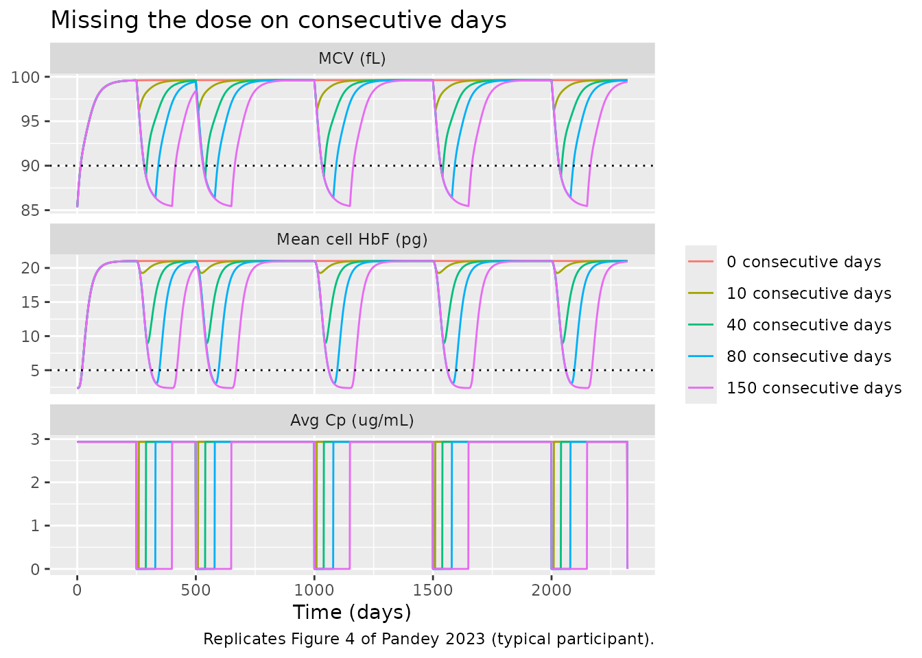
fig4_tbt <- tbt(fig4)
fig4_tbt |>
  dplyr::rename(Regimen = regimen, "%miss" = pct_miss, "%tbt MCV" = tbt_mcv, "%tbt HbF" = tbt_hbf) |>
knitr::kable(digits = 0, caption = "Figure 4 regimens. Pandey 2023 reports %miss 0/2/9/17/32 with %tbt MCV 0/0/7/20/36 and HbF 0/0/0/11/28.")| Regimen | %miss | %tbt MCV | %tbt HbF |
|---|---|---|---|
| 0 consecutive days | 0 | 1 | 1 |
| 10 consecutive days | 2 | 1 | 1 |
| 40 consecutive days | 9 | 3 | 1 |
| 80 consecutive days | 17 | 13 | 9 |
| 150 consecutive days | 32 | 29 | 24 |
# The %miss values follow from the design and must match the paper's.
stopifnot(all(abs(fig4_tbt$pct_miss - c(0, 2, 9, 17, 32)) < 1))
# Paper: %tbt for MCV is 0 for 10 consecutive missed days and grows with
# longer blocks. The simulation is deterministic (no random draws).
stopifnot(
  fig4_tbt$tbt_mcv[2] < 1,
  all(diff(fig4_tbt$tbt_mcv) >= 0),
  fig4_tbt$tbt_mcv[5] > fig4_tbt$tbt_mcv[3]
)
The 10-day blocks barely move either biomarker, while 80- and 150-day blocks let MCV fall back towards its 85 fL baseline and spend a growing share of time below 90 fL, as in Figure 4. The typical participant’s baseline mean cell HbF (2.4 pg) is below the 5 pg threshold, so %tbt for HbF also includes the first weeks of treatment; the paper’s representative participant started near 2 pg as well.
Interspersed vs. consecutive missed doses (Figure 5)
From day 200 a dose is missed after every four doses (4:1), compared with the five 80-day blocks of Figure 4. Both miss about 400 doses (%miss 17-18).
days_all <- seq(0, n_days - 1)
four_one <- days_all[!(days_all >= 200 & (days_all - 200) %% 5 == 4)]
fig5_ev <- dplyr::bind_rows(
  make_regimen(1L, "4:1 pattern", four_one, n_days),
  make_regimen(2L, "80 consecutive days", setdiff(days_all, missed_blocks(80)), n_days)
)
fig5 <- solve_days(fig5_ev)
plot_bio(fig5, "Interspersed vs. consecutive nonadherence", "Replicates Figure 5 of Pandey 2023 (typical participant).")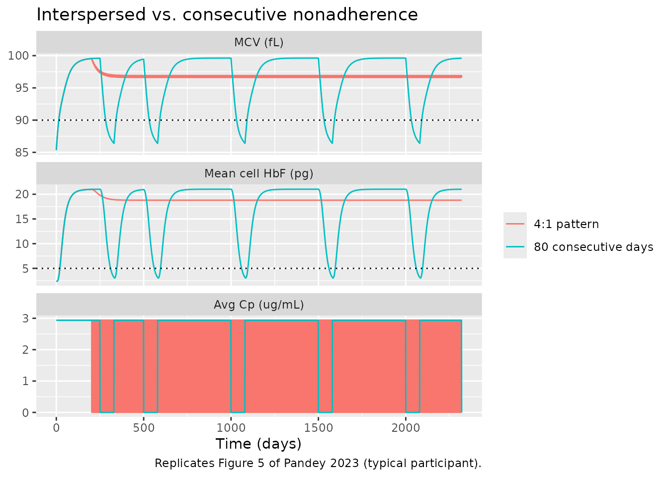
fig5_tbt <- tbt(fig5)
fig5_tbt |>
  dplyr::rename(Regimen = regimen, "%miss" = pct_miss, "%tbt MCV" = tbt_mcv, "%tbt HbF" = tbt_hbf) |>
knitr::kable(digits = 0, caption = "Figure 5 regimens. Pandey 2023 reports %tbt 0 (both biomarkers) for 4:1 and MCV 20 / HbF 11 for 80 consecutive days.")| Regimen | %miss | %tbt MCV | %tbt HbF |
|---|---|---|---|
| 4:1 pattern | 18 | 1 | 1 |
| 80 consecutive days | 17 | 13 | 9 |
four <- fig5_tbt[fig5_tbt$regimen == "4:1 pattern", ]
block <- fig5_tbt[fig5_tbt$regimen == "80 consecutive days", ]
stopifnot(
  abs(four$pct_miss - 18) < 1, abs(block$pct_miss - 17) < 1,
  # The paper's key finding: spread-out misses keep MCV above threshold,
  # consecutive misses do not.
  four$tbt_mcv < 1,
  block$tbt_mcv > 5
)
As in the paper, the same number of missed doses keeps MCV above 90 fL when spread out and drops it below the threshold for weeks when taken as long breaks.
Daily adherence probability (Figure 6)
Each day the dose is taken with probability p, drawn once per regimen with R’s random number generator.
set.seed(20230516)
probs <- c(0, 0.25, 0.5, 0.75, 1)
fig6_ev <- dplyr::bind_rows(lapply(seq_along(probs), function(i) {
  taken <- days_all[stats::runif(length(days_all)) < probs[i]]
  make_regimen(i, sprintf("p = %.2f", probs[i]), taken, n_days)
}))
fig6 <- solve_days(fig6_ev) |>
  dplyr::mutate(regimen = factor(regimen, levels = sprintf("p = %.2f", probs)))
plot_bio(fig6, "Fixed daily probability of taking the dose", "Replicates Figure 6 of Pandey 2023 (typical participant).")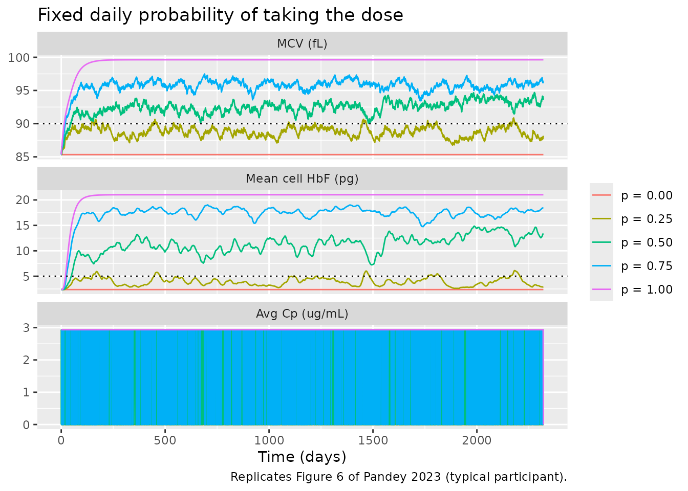
fig6_late <- fig6 |>
  dplyr::filter(time >= 1000) |>
  dplyr::group_by(regimen) |>
  dplyr::summarise(mean_mcv = mean(MCV), mean_hbf = mean(hbf_mc), .groups = "drop")
knitr::kable(fig6_late, digits = 1, caption = "Mean MCV and mean cell HbF after day 1000 by adherence probability.")| regimen | mean_mcv | mean_hbf |
|---|---|---|
| p = 0.00 | 85.3 | 2.4 |
| p = 0.25 | 88.7 | 3.9 |
| p = 0.50 | 92.8 | 12.1 |
| p = 0.75 | 95.8 | 17.5 |
| p = 1.00 | 99.6 | 21.0 |
# MCV rises with adherence, roughly in proportion to the fraction of days
# dosed (the MCV equation is linear in the daily average concentration); the
# p = 1 vs. p = 0 gap is ~14 fL, far above the variation between draws.
stopifnot(
  fig6_late$mean_mcv[5] - fig6_late$mean_mcv[1] > 10,
  fig6_late$mean_mcv[4] > fig6_late$mean_mcv[2],
  fig6_late$mean_hbf[5] > fig6_late$mean_hbf[1]
)
Per-participant estimates (Tables S2 and S4)
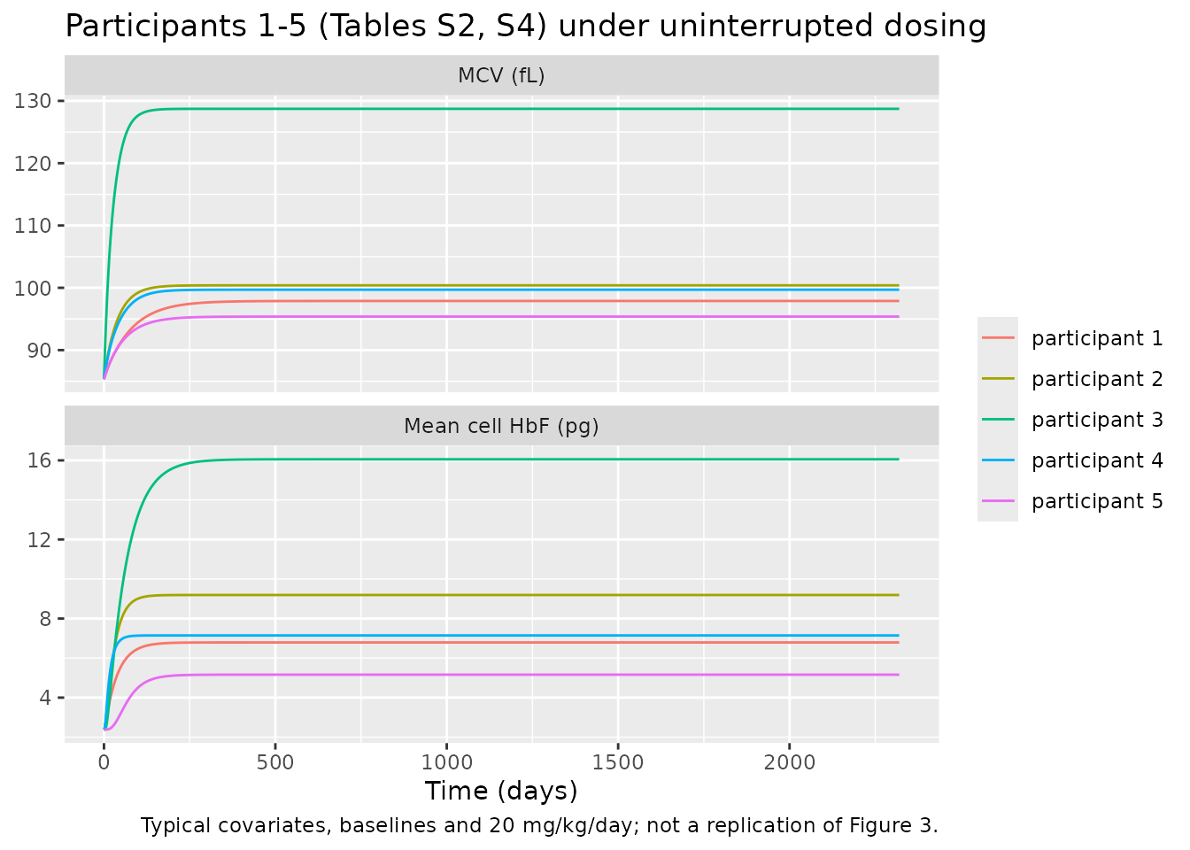
Pandey 2023 re-estimated the MCV and HbF parameters of each of the 40 participants after correcting their dosing profiles for inferred nonadherence (Tables S2 and S4; Tables S1 and S3 hold the fits to the uncorrected pharmacy profiles). Most of their medians are within a factor of two of the Pandey 2022 cohort medians used as the typical values. The feedback parameter Psi_e and the stem-cell kill potency Kdse,50 differ several-fold: the 40 refitted participants are a selected subgroup, and Kdse,50 is poorly determined because both values sit far below the daily average concentration of about 40 uM, where stem-cell kill is near its maximum.
s2 <- read.table(header = TRUE, text = "
id psi_rbc gamma_rbc kdsemax kdse50 kte kdemax kde50 alpha_mcv
1 9.0E+11 0.12 0.068 41.72 0.2913 0.014 859.49 0.325
2 7.2E+12 1.91 0.110 54.89 0.5474 0.027 948.49 0.390
3 1.8E+11 1.29 0.025 2.13 0.2270 0.040 516.24 1.124
4 8.0E+12 1.81 0.046 26.60 0.1588 0.025 809.04 0.372
5 1.1E+12 1.66 0.015 59.86 0.2146 0.018 955.42 0.260
6 3.3E+11 2.20 0.021 0.64 0.1212 0.033 439.12 0.438
7 1.7E+12 0.26 0.314 27.64 0.2026 0.011 775.36 0.631
8 1.9E+11 1.71 0.080 0.03 0.4718 0.024 563.99 0.340
9 3.3E+12 0.13 0.022 59.50 0.8048 0.016 573.20 0.263
10 1.0E+13 3.62 0.579 20.33 0.2130 0.002 376.48 2.256
11 6.2E+12 1.00 0.293 24.13 0.5333 0.026 503.33 0.851
12 3.8E+12 2.31 0.244 19.15 0.3735 0.113 942.31 0.445
13 2.1E+11 1.41 0.128 3.41 0.6147 0.026 981.00 0.670
14 5.1E+11 3.12 0.421 2.28 0.5942 0.040 127.42 0.849
15 1.8E+12 2.26 0.491 32.37 0.5993 0.040 703.21 0.635
16 4.6E+10 2.01 0.591 46.92 0.6301 0.032 753.32 0.545
17 4.9E+10 1.10 0.264 3.72 0.2345 0.026 876.26 0.591
18 1.9E+11 0.15 0.037 44.54 0.0782 0.009 915.61 0.440
19 1.8E+12 1.03 0.198 42.66 0.2206 0.032 443.52 0.398
20 2.0E+12 0.37 0.009 56.08 0.2553 0.216 328.39 0.483
21 6.4E+11 2.44 0.428 91.43 0.5447 0.045 888.80 0.508
22 8.3E+11 1.65 0.001 3.73 0.0050 0.015 956.24 0.324
23 2.9E+11 3.71 0.089 4.18 0.0005 0.068 956.34 0.173
24 1.5E+12 0.29 0.025 14.64 0.0809 0.005 233.14 0.438
25 1.2E+12 0.44 0.017 4.51 0.0341 0.006 980.07 0.486
26 2.2E+12 1.61 0.633 22.86 0.7050 0.037 480.76 0.265
27 1.2E+12 3.98 0.000 51.13 0.0072 0.005 129.90 0.669
28 4.9E+11 2.22 0.021 34.73 0.1636 0.069 650.60 0.551
29 5.0E+12 1.93 0.011 40.24 0.1265 0.093 650.36 0.171
30 6.5E+11 2.33 0.694 61.54 0.4912 0.045 57.03 0.313
31 4.6E+11 1.72 0.024 17.91 0.5926 0.018 808.83 0.733
32 8.4E+11 1.93 0.228 2.65 0.2772 0.022 429.97 0.668
33 2.5E+12 2.74 0.537 41.92 0.2169 0.038 98.51 0.365
34 4.3E+12 0.17 0.168 0.96 0.4490 0.050 639.07 0.447
35 2.4E+10 1.28 0.589 20.14 0.3184 0.017 238.67 0.452
36 1.0E+13 0.41 1.000 1.04 0.0212 0.000 19.99 21.637
37 1.8E+11 1.21 0.605 45.75 0.2641 0.121 102.53 0.600
38 9.8E+10 1.94 0.041 2.61 0.3784 0.100 670.67 0.431
39 3.6E+12 1.32 0.864 2.27 0.1565 0.003 1.76 1.597
40 1.0E+10 0.87 0.000 0.03 0.0006 0.014 331.64 0.363
")
s4 <- read.table(header = TRUE, text = "
id kmet kmmet kdi kaf kaf50 hill_hbf kdf
1 0.565 2.75 0.735 5.40 5.12 1.93 0.027
2 3.589 19.67 0.161 2.17 100.00 1.03 0.039
3 0.584 29.25 0.073 0.27 2.22 3.25 0.018
4 4.124 99.07 0.064 4.77 23.26 1.50 0.407
5 4.908 99.02 0.026 0.68 69.14 3.06 0.075
6 0.461 11.00 0.042 4.39 28.80 2.25 0.036
7 2.320 98.54 0.003 7.88 90.71 2.17 0.736
8 0.013 4.39 0.012 3.94 0.65 1.95 0.447
9 9.963 99.93 0.019 0.49 82.04 3.40 0.064
10 8.975 33.27 0.284 0.55 48.54 3.18 0.004
11 1.069 33.84 0.014 2.37 32.54 3.81 0.203
12 0.508 17.10 0.043 0.14 7.25 0.99 0.025
13 0.003 0.42 0.020 4.42 0.50 1.09 0.121
14 1.703 54.23 0.020 2.44 25.83 3.50 0.187
15 0.006 14.12 0.025 2.80 0.49 1.07 0.128
16 0.630 26.64 0.093 9.96 10.69 3.24 0.103
17 2.030 99.55 0.029 5.46 100.00 1.38 0.080
18 1.511 40.25 0.070 0.08 12.56 3.99 0.006
19 8.910 99.01 0.042 0.13 67.01 3.51 0.024
20 0.259 30.66 0.065 3.04 3.54 3.02 0.138
21 1.363 92.03 0.013 2.30 33.86 2.50 0.212
22 0.101 24.97 0.008 0.93 4.94 3.37 0.159
23 1.275 100.00 0.209 5.05 20.89 1.31 0.054
24 0.167 9.33 0.005 0.08 12.52 3.73 0.016
25 0.026 86.63 0.005 4.96 0.66 2.54 0.578
26 7.778 99.01 0.018 0.48 93.15 3.99 0.103
27 0.002 3.31 0.009 0.29 0.30 2.20 0.013
28 1.616 95.36 0.008 9.98 59.92 2.98 0.550
29 9.824 85.81 0.516 8.75 99.44 2.03 0.013
30 6.066 66.95 1.000 9.64 8.85 1.99 0.151
31 1.353 95.01 0.055 0.25 7.64 1.70 0.016
32 0.607 2.86 0.291 5.26 20.95 1.49 0.012
33 2.814 97.80 0.044 5.97 71.79 2.07 0.099
34 2.826 3.48 0.168 1.32 39.93 1.90 0.020
35 0.033 9.56 0.000 5.34 23.87 1.52 0.233
36 9.294 10.60 0.311 1.05 47.70 3.02 0.032
37 0.483 37.21 0.008 1.64 34.19 2.39 0.186
38 2.988 11.14 0.054 1.42 58.94 2.83 0.074
39 7.390 87.19 0.041 0.10 10.94 2.58 0.018
40 7.699 96.47 0.031 0.27 94.71 0.65 0.017
")
stopifnot(nrow(s2) == 40, nrow(s4) == 40)
# psi_rbc is tabulated in cells/L; the model carries 10^12 cells/L.
s2$psi_rbc <- s2$psi_rbc / 1e12
typical <- th[c(names(s2)[-1], names(s4)[-1])]
summ <- dplyr::bind_rows(
  lapply(names(s2)[-1], function(p) data.frame(parameter = p, x = s2[[p]])),
  lapply(names(s4)[-1], function(p) data.frame(parameter = p, x = s4[[p]]))
) |>
  dplyr::group_by(parameter) |>
  dplyr::summarise(q1 = quantile(x, 0.25), median = median(x), q3 = quantile(x, 0.75), .groups = "drop") |>
  dplyr::mutate(typical_value = typical[parameter]) |>
  dplyr::arrange(match(parameter, names(typical)))
summ |>
  dplyr::rename(
    Parameter = parameter, "Q1 (2023)" = q1, "Median (2023)" = median,
    "Q3 (2023)" = q3, "Packaged typical value (2022 median)" = typical_value
  ) |>
knitr::kable(digits = 3, caption = "Corrected per-participant estimates of Pandey 2023 (Tables S2, S4) vs. the packaged typical values. psi_rbc in 10^12 cells/L.")| Parameter | Q1 (2023) | Median (2023) | Q3 (2023) | Packaged typical value (2022 median) |
|---|---|---|---|---|
| psi_rbc | 0.270 | 1.000 | 2.700 | 0.22 |
| gamma_rbc | 0.968 | 1.655 | 2.205 | 1.60 |
| kdsemax | 0.024 | 0.119 | 0.444 | 0.17 |
| kdse50 | 3.220 | 21.595 | 43.130 | 0.43 |
| kte | 0.149 | 0.245 | 0.502 | 0.20 |
| kdemax | 0.015 | 0.026 | 0.041 | 0.03 |
| kde50 | 330.828 | 606.135 | 863.683 | 310.00 |
| alpha_mcv | 0.364 | 0.450 | 0.643 | 0.37 |
| kmet | 0.478 | 1.437 | 4.320 | 1.20 |
| kmmet | 11.105 | 35.525 | 95.637 | 27.00 |
| kdi | 0.014 | 0.042 | 0.078 | 0.03 |
| kaf | 0.488 | 2.335 | 5.102 | 1.50 |
| kaf50 | 7.542 | 24.850 | 61.692 | 13.00 |
| hill_hbf | 1.655 | 2.320 | 3.195 | 3.20 |
| kdf | 0.020 | 0.074 | 0.166 | 0.07 |
To simulate one of these participants, override the parameters on the log scale. Below, the corrected estimates of participants 1-5 are run through the typical participant’s covariates, baselines and uninterrupted dosing, so the spread reflects the parameters only (the participants’ own baselines and dosing records are not published).
ids <- 1:5
pars <- dplyr::inner_join(s2, s4, by = "id") |>
  dplyr::filter(id %in% ids) |>
  dplyr::mutate(dplyr::across(-id, log)) |>
  dplyr::rename_with(~ paste0("l", .x), -id)
part_ev <- dplyr::bind_rows(lapply(ids, function(i) {
  make_regimen(i, sprintf("participant %d", i), days_all, n_days)
}))
part_sim <- rxode2::rxSolve(mod,
  events = dplyr::arrange(part_ev, id, time, dplyr::desc(evid)),
  params = dplyr::select(pars, -id), keep = "regimen", maxsteps = 1e6, hmax = 0.1
) |>
  as.data.frame() |>
  dplyr::filter(time == round(time))
# Each participant's own kte must be in force (params rows map to ids in order).
kte_used <- part_sim |> dplyr::distinct(id, kte)
stopifnot(all(abs(kte_used$kte / s2$kte[match(kte_used$id, s2$id)] - 1) < 1e-8))
part_sim |>
  dplyr::select(time, regimen, `MCV (fL)` = MCV, `Mean cell HbF (pg)` = hbf_mc) |>
  tidyr::pivot_longer(-c(time, regimen)) |>
  ggplot(aes(time, value, colour = regimen)) +
  geom_line() +
  facet_wrap(~name, ncol = 1, scales = "free_y") +
  labs(
    x = "Time (days)", y = NULL, colour = NULL,
    title = "Participants 1-5 (Tables S2, S4) under uninterrupted dosing",
    caption = "Typical covariates, baselines and 20 mg/kg/day; not a replication of Figure 3."
  )
Assumptions and deviations
- Typical values come from the parent paper. Pandey 2023 reports only per-participant estimates. The packaged values are the HUSTLE cohort central values of Pandey 2022, which fitted the same equations: means for the PK (Table 2) and medians for the pharmacodynamics (Tables 3 and 5). The per-parameter medians of the 2023 corrected estimates are compared with them in the table above. A set of per-parameter medians is not itself a fitted individual.
- PK of the 2023 participants is not published. Pandey 2023 reuses each participant’s PK fit from Pandey 2022 without tabulating it; the cohort means of Pandey 2022 Table 2 are used.
-
Units of the daily average concentration. Both
papers plot the daily average concentration in ug/mL, while every
concentration parameter of the pharmacodynamic model is reported per uM.
The model converts with the molar mass of hydroxyurea (76.05 g/mol),
which neither paper states. Using ug/mL directly would make the MCV rise
alpha Cabout 13-fold smaller (0.37 x 3 = 1 fL instead of 14 fL at 20 mg/kg), far below the 18 fL rise from baseline to 6 months in Pandey 2022 Table 1. -
Nadler blood volume. Both papers print the height
term of the Nadler equation as
height (cm)^3, which gives blood volumes of about 10^5 L. The model uses height in metres, as in Nadler’s equation; this reproduces the mean plasma volume of 1.77 L in Pandey 2022 Table 2 (1.89 L for the typical participant here). -
Initial conditions. The papers set the initial
conditions from each participant’s baseline data. The red-cell chain
starts at its pre-treatment steady state,
Nse(0) = Ne1(0) = Ne2(0) = Ne3(0) = kde,max Ne(0) / kte, which is the state implied by the printedkpe,maxformula; the HbF intermediate starts at zero. Baselines are parameters whose typical values are the HUSTLE baseline means (Pandey 2022 Table 1). -
Daily average concentration. The source simulates
the PK model each day and averages it. The model uses the equivalent
closed form
F D / (ke Vp) / 1 dayfor the day after each dose and zero for a day without one; the check above shows it equals the integral of the simulated profile. It assumes once-daily dosing and a dose that is cleared within the day (true for the typical half-life of 1.3 h). -
Solver settings. Multi-year daily-dosing
simulations are run with
hmax = 0.1(day) so the integrator resolves each day’s absorption peak. - Hematocrit and body size are covariates supplied by the user; the source updated them daily from clinic data. They are held constant here.
- No variability. The individual weighted-least-squares fits carry no between-subject variability or residual error model.
- Figures 4-6 use a typical participant at 20 mg/kg/day; the representative participant of the paper (covariates, baselines, parameters and dose history) is not identified, so values differ while the patterns match.
- No erratum to either paper was found (checked 2026-10-26).