Dalbavancin (Benavent 2025)
Source:vignettes/articles/Benavent_2025_dalbavancin.Rmd
Benavent_2025_dalbavancin.RmdModel and source
- Citation: Benavent E, Lora-Tamayo J, Ulldemolins M, Pons-Oltra P, Gregoire M, Mancheno-Losa M, Hernandez-Jimenez P, Melendez-Carmona MA, Casals V, Roberts JA, Rigo-Bonnin R, Murillo O. Efficacy, safety, and population pharmacokinetics of a single 1500 mg dose of dalbavancin for short-term therapy in patients with chronic prosthetic joint infections. Antimicrob Agents Chemother. 2025;69(12):e00773-25. doi:10.1128/aac.00773-25
- Article: Antimicrob Agents Chemother 2025;69(12):e00773-25 (open access, CC BY 4.0; PMC12691635)
Dalbavancin is a lipoglycopeptide with a terminal half-life near two weeks, so a single infusion can cover weeks of therapy. Benavent 2025 asked whether one 1500 mg dose is enough to finish the four-week antibiotic course that follows first-stage surgery for a chronic prosthetic joint infection, where the infected implant is removed, a vancomycin- plus gentamicin-loaded cement spacer is put in, and a new prosthesis is implanted at a second operation months later. Twenty patients were treated; eighteen contributed plasma concentrations to a population PK model, which was then used for Monte Carlo target-attainment simulations.
The model is deliberately simple: one compartment, intravenous infusion, first-order elimination, interindividual variability on both clearance and volume, proportional residual error, and no covariates – the covariate search improved nothing, so the structural model is the final model.
# rxode2::rxode() resolves the model function to an rxUi without depending on
# ini()/model() being attached.
mod <- rxode2::rxode(readModelDb("Benavent_2025_dalbavancin"))
#> ℹ parameter labels from comments will be replaced by 'label()'
mod
#>  ── rxode2-based free-form 1-cmt ODE model ──────────────────────────────────────
#>  ── Initalization: ──
#> Fixed Effects ($theta):
#>       lvc       lcl    propSd
#>  2.884801 -3.324236  0.120000
#>
#> Omega ($omega):
#>        etalvc etalcl
#> etalvc   0.04 0.0000
#> etalcl   0.00 0.0841
#> attr(,"lotriLabels")
#> [1] "Table 2, 'IIV V (SD)' = 0.200 (27.4% RSE); bootstrap median 0.200 (95% CI 0.061-0.280). Squared to a variance."
#> [2] "Table 2, 'IIV CL (SD)' = 0.290 (20.8% RSE); bootstrap median 0.280 (95% CI 0.150-0.380). Squared to a variance."
#> attr(,"lotriFix")
#>        etalvc etalcl
#> etalvc  FALSE  FALSE
#> etalcl  FALSE  FALSE
#>
#> States ($state or $stateDf):
#>   Compartment Number Compartment Name
#> 1                  1          central
#>  ── μ-referencing ($muRefTable): ──
#>   theta    eta level
#> 1   lvc etalvc    id
#> 2   lcl etalcl    id
#>
#>  ── Model (Normalized Syntax): ──
#> function() {
#>     compartmentData <- list(central = list(analyte = "dalbavancin",
#>         units = "mg", specimen = "plasma", verified = TRUE))
#>     covariateData <- list()
#>     covariatesDataExcluded <- list(AGE = list(description = "Age",
#>         units = "years", type = "continuous", notes = "Screened on the structural model but not retained. Median 75.5 years, interquartile interval 69-79 years (Benavent 2025 Results, first paragraph)."),
#>         SEXF = list(description = "Sex (1 = female, 0 = male)",
#>             units = "(binary)", type = "binary", notes = "Printed as 'gender' in Benavent 2025 Methods; screened but not retained. 70% of the 20 enrolled patients were female (n = 14; Results, first paragraph). Recorded here on the canonical female-indicator convention."),
#>         HT = list(description = "Body height", units = "cm",
#>             type = "continuous", notes = "Screened but not retained (Benavent 2025 Methods). The paper does not print a cohort height summary in the main text."),
#>         WT = list(description = "Total body weight", units = "kg",
#>             type = "continuous", notes = "Screened but not retained (Benavent 2025 Methods). The paper does not print a cohort weight summary in the main text, and no allometric scaling is applied; the packaged V and CL are absolute values for this elderly cohort."),
#>         BMI = list(description = "Body mass index", units = "kg/m^2",
#>             type = "continuous", notes = "Screened but not retained (Benavent 2025 Methods). The paper does not print a cohort body-mass-index summary in the main text."),
#>         CRCL = list(description = "Renal function: BSA-normalized glomerular filtration rate and, separately, baseline creatinine clearance",
#>             units = "mL/min", type = "continuous", notes = "Benavent 2025 screened TWO renal-function covariates as separate candidates -- glomerular filtration rate (their reference 19) and baseline creatinine clearance by the Cockcroft-Gault-style equation of their reference 20 -- and retained neither. Both fold onto the single canonical CRCL column, whose register entry explicitly spans creatinine-based estimated GFR and measured creatinine clearance. The cohort had uniformly preserved renal function (median glomerular filtration rate 90 mL/min, interquartile interval 75.8-96.3 mL/min; Results, first paragraph), which is the likely reason no renal effect was identifiable. The paper reports the GFR summary without stating whether it is BSA-normalized, so the units above are given as the printed mL/min. The Discussion nevertheless attributes this cohort's 30% lower clearance versus healthy volunteers partly to its lower creatinine clearance, i.e. the effect is believed real but was not estimable in 18 patients spanning a narrow renal range."),
#>         ALB = list(description = "Serum albumin on the day of sampling",
#>             units = "g/L", type = "continuous", notes = "Screened but not retained (Benavent 2025 Methods, which specifies 'albumin serum concentrations on the day of sampling', i.e. a time-varying candidate). The cohort had normal albumin throughout: median 45 g/L, interquartile interval 38-47 g/L (Results, first paragraph). The Discussion attributes part of this cohort's lower clearance to its physiological albumin relative to the comparator populations."))
#>     description <- "One-compartment population PK model with intravenous infusion and first-order linear elimination for TOTAL plasma dalbavancin after a SINGLE 1500 mg dose given as sequencing therapy to elderly adults with chronic Gram-positive prosthetic joint infection managed by two-stage exchange with vancomycin/gentamicin-loaded cement spacers. Interindividual variability was estimated on both clearance and volume; residual error is proportional. No covariate improved the fit, so the structural model IS the final model: age, sex, height, body weight, body mass index, glomerular filtration rate, baseline creatinine clearance and same-day serum albumin were all screened and rejected. The model returns TOTAL dalbavancin Cc; the paper's PK/PD target attainment analysis derives unbound exposure by scaling Cc with a free fraction swept over four theoretical protein-binding scenarios (93, 95, 97 and 99 percent), so no single free fraction is packaged here. Clearance is about 30 percent lower than reported for healthy volunteers and younger patients with acute infection (0.036 vs 0.050 L/h), which the authors attribute to the cohort's older age, physiological albumin and lower creatinine clearance."
#>     population <- list(species = "human", n_subjects = 18L, n_studies = 1L,
#>         age_median = "75.5 years", age_range = "interquartile interval 69-79 years",
#>         sex_female_pct = 70, race_ethnicity = "Not reported; two-centre Spanish cohort.",
#>         disease_state = "Chronic prosthetic joint infection caused by low-virulence Gram-positive bacteria susceptible to dalbavancin, managed by two-stage prosthetic exchange with a vancomycin- plus gentamicin-loaded cement spacer. Affected joints: hip 55% (n = 11), knee 30% (n = 6), shoulder 10% (n = 2), ankle 5% (n = 1). Isolates (Table 1, 24 isolates): coagulase- negative staphylococci 70.8% (Staphylococcus epidermidis 50%, S. lugdunensis 4.2%, other CoNS 16.7%), Cutibacterium acnes 25%, Enterococcus faecalis 4.2%; four polymicrobial infections.",
#>         dose_range = "A single 1500 mg intravenous dose of dalbavancin, given as a 30 min short infusion at Hospital 12 de Octubre or a 2 h extended infusion at Hospital Universitari de Bellvitge, after a median 11.5 days (interquartile interval 10-16) of prior intravenous therapy (vancomycin 75%, daptomycin 25%; switched to an oxazolidinone before dalbavancin in 30% of cases).",
#>         regions = "Spain (Hospital Universitari de Bellvitge, Barcelona; Hospital Universitario 12 de Octubre, Madrid)",
#>         renal_function = "Uniformly preserved: median glomerular filtration rate 90 mL/min, interquartile interval 75.8-96.3 mL/min (Results, first paragraph). No patient had renal impairment, and no change in renal function occurred during follow-up.",
#>         notes = "Retrospective, observational, two-centre clinical and PK study run 1 January 2022 to 31 May 2023 (ethics reference EOM017/23). Twenty patients were enrolled and reported for the efficacy and safety endpoints; the population PK model was fitted to TOTAL plasma dalbavancin from 18 of them (Results, 'Population pharmacokinetic analysis'), each contributing 1-3 concentrations, so the analysis dataset holds between 18 and 54 observations -- the exact count is given only in supplementary Table S2, which was not retrievable (see the vignette Errata). Sampling was opportunistic at weekly-to-biweekly outpatient visits through week 4 post-dose rather than on a fixed schedule. Total dalbavancin was measured by UHPLC-MS/MS with a lower limit of quantification of 1.0 mg/L over a 1.0-250 mg/L measuring interval, imprecision <= 8.6% and absolute relative bias <= 7.3%. Estimation was SAEM in Monolix 2024R1; the final model was checked by prediction-corrected VPC (500 simulations) and by nonparametric bootstrap (n = 1000). Serum albumin was normal throughout (median 45 g/L, interquartile interval 38-47 g/L).")
#>     reference <- "Benavent E, Lora-Tamayo J, Ulldemolins M, Pons-Oltra P, Gregoire M, Mancheno-Losa M, Hernandez-Jimenez P, Melendez-Carmona MA, Casals V, Roberts JA, Rigo-Bonnin R, Murillo O. Efficacy, safety, and population pharmacokinetics of a single 1500 mg dose of dalbavancin for short-term therapy in patients with chronic prosthetic joint infections. Antimicrob Agents Chemother. 2025;69(12):e00773-25. doi:10.1128/aac.00773-25"
#>     units <- list(time = "h", dosing = "mg", concentration = "mg/L")
#>     vignette <- "Benavent_2025_dalbavancin"
#>     ini({
#>         lvc <- 2.88480071284671
#>         label("Central volume of distribution (L)")
#>         lcl <- -3.32423634052603
#>         label("Clearance (L/h)")
#>         propSd <- c(0, 0.12)
#>         label("Proportional residual error (fraction)")
#>         etalvc ~ 0.04
#>         label("Table 2, 'IIV V (SD)' = 0.200 (27.4% RSE); bootstrap median 0.200 (95% CI 0.061-0.280). Squared to a variance.")
#>         etalcl ~ 0.0841
#>         label("Table 2, 'IIV CL (SD)' = 0.290 (20.8% RSE); bootstrap median 0.280 (95% CI 0.150-0.380). Squared to a variance.")
#>     })
#>     model({
#>         vc <- exp(lvc + etalvc)
#>         cl <- exp(lcl + etalcl)
#>         kel <- cl/vc
#>         d/dt(central) <- -kel * central
#>         Cc <- central/vc
#>         Cc ~ prop(propSd)
#>     })
#> }
Population
Eighteen of the twenty enrolled patients contributed total plasma dalbavancin concentrations, each supplying one to three samples drawn opportunistically at weekly-to-biweekly outpatient visits through week four. The cohort is elderly (median age 75.5 years, interquartile interval 69-79) and predominantly female (70%, n = 14). Renal function and albumin were uniformly normal – median glomerular filtration rate 90 mL/min (interquartile interval 75.8-96.3) and median albumin 45 g/L (38-47) – which matters, because it is the most likely reason no covariate reached significance.
Infection involved a hip prosthesis in 55% of patients, knee in 30%, shoulder in 10% and ankle in 5%. Coagulase-negative staphylococci accounted for 70.8% of the 24 isolates (Table 1), with Cutibacterium acnes at 25% and Enterococcus faecalis at 4.2%; four infections were polymicrobial. Every patient received a single 1500 mg intravenous dose after a median 11.5 days of prior intravenous therapy, given as a 30-minute infusion at one hospital and a 2-hour infusion at the other.
The same information is available programmatically:
str(rxode2::rxode(readModelDb("Benavent_2025_dalbavancin"))$population)
#> ℹ parameter labels from comments will be replaced by 'label()'
#> List of 12
#>  $ species       : chr "human"
#>  $ n_subjects    : int 18
#>  $ n_studies     : int 1
#>  $ age_median    : chr "75.5 years"
#>  $ age_range     : chr "interquartile interval 69-79 years"
#>  $ sex_female_pct: num 70
#>  $ race_ethnicity: chr "Not reported; two-centre Spanish cohort."
#>  $ disease_state : chr "Chronic prosthetic joint infection caused by low-virulence Gram-positive bacteria susceptible to dalbavancin, m"| __truncated__
#>  $ dose_range    : chr "A single 1500 mg intravenous dose of dalbavancin, given as a 30 min short infusion at Hospital 12 de Octubre or"| __truncated__
#>  $ regions       : chr "Spain (Hospital Universitari de Bellvitge, Barcelona; Hospital Universitario 12 de Octubre, Madrid)"
#>  $ renal_function: chr "Uniformly preserved: median glomerular filtration rate 90 mL/min, interquartile interval 75.8-96.3 mL/min (Resu"| __truncated__
#>  $ notes         : chr "Retrospective, observational, two-centre clinical and PK study run 1 January 2022 to 31 May 2023 (ethics refere"| __truncated__
Source trace
Every value in the model file comes from Table 2 of the paper, which is reproduced in full here. The paper prints no other parameter table.
| Quantity | Model file | Source location | Published value |
|---|---|---|---|
| Central volume | lvc = log(17.9) | Table 2, ‘V (L)’ | 17.9 L (6.2% RSE) [18.1% shrinkage]; bootstrap 18.0 (16.0-20.3) |
| Clearance | lcl = log(0.036) | Table 2, ‘CL (L/h)’ | 0.036 L/h (8.2% RSE) [12.6% shrinkage]; bootstrap 0.037 (0.031-0.043) |
| IIV on volume | etalvc ~ 0.200^2 | Table 2, ‘IIV V (SD)’ | 0.200 SD (27.4% RSE); bootstrap 0.200 (0.061-0.280) |
| IIV on clearance | etalcl ~ 0.290^2 | Table 2, ‘IIV CL (SD)’ | 0.290 SD (20.8% RSE); bootstrap 0.280 (0.150-0.380) |
| Proportional residual | propSd = 0.120 | Table 2, ‘b (proportional)’ | 0.120 (28.6% RSE); bootstrap 0.110 (0.053-0.170) |
| Structure | 1-cmt IV, kel | Results, ‘Population pharmacokinetic analysis’ | ‘one-compartment model with intravenous infusion and first-order linear elimination’ |
| Error model | Cc ~ prop(propSd) | Results, ‘Population pharmacokinetic analysis’ | ‘the residual error was modeled as proportional’ |
| IIV distribution | exp(l* + eta) | Methods, ‘Structural model building’ | ‘log-normally distributed … IIV was described using an exponential model’ |
| Covariates | none | Results, ‘Population pharmacokinetic analysis’ | ‘The covariate analysis did not result in model improvements’ |
Monolix reports omega on the standard-deviation scale, and Table 2
labels the rows IIV V (SD) / IIV CL (SD) with
footnote a spelling out “SD, standard deviation”, so the model
file squares the printed values to variances. This is the single most
consequential reading in the extraction, and the paper leaves no room
for doubt about it.
Structural check against closed form
For a one-compartment model with no covariates the typical-value profile has an exact closed form, so this check is deterministic – it contains no random draw and the bounds can be tight.
DOSE <- 1500      # mg, single intravenous dose
TINF <- 0.5       # h, 30 min infusion used in the paper's Monte Carlo

typ  <- rxode2::zeroRe(mod)
obs_t <- sort(unique(c(
  seq(0, 4, by = 0.1),        # resolve the end-of-infusion peak
  seq(6, 48, by = 6),
  seq(72, 2520, by = 24),     # out to 15 weeks so AUCinf is well determined
  seq(504, 528, by = 2),      # the three 24 h PK/PD windows (days 21, 27, 35)
  seq(648, 672, by = 2),
  seq(840, 864, by = 2)
)))
ev_typ <- rxode2::et(amt = DOSE, dur = TINF, cmt = "central") |> rxode2::et(obs_t)
sim_typ <- as.data.frame(rxode2::rxSolve(typ, ev_typ))
#> ℹ omega/sigma items treated as zero: 'etalvc', 'etalcl'

cl_t  <- 0.036
vc_t  <- 17.9
kel_t <- cl_t / vc_t

# Closed form for a constant-rate infusion of duration TINF, evaluated after
# the infusion has stopped.
cc_closed <- function(t) {
  (DOSE / (cl_t * TINF)) * (1 - exp(-kel_t * TINF)) * exp(-kel_t * (t - TINF))
}

chk <- sim_typ |>
  filter(time >= TINF) |>
  mutate(closed = cc_closed(time), pct = 100 * (Cc - closed) / closed)

c(max_abs_pct_diff = max(abs(chk$pct)),
  cmax_mg_L        = max(sim_typ$Cc),
  half_life_days   = log(2) / kel_t / 24)
#> max_abs_pct_diff        cmax_mg_L   half_life_days
#>     4.360808e-05     8.375676e+01     1.436034e+01
stopifnot(
  # Deterministic: solver vs closed form, so this is pure numerical error and a
  # tight bound is correct. A mis-transcribed V, CL or infusion duration breaks
  # it immediately.
  max(abs(chk$pct)) < 0.5,
  # Cmax = (Dose / (CL * TINF)) * (1 - exp(-kel * TINF)); 83.8 mg/L.
  abs(max(sim_typ$Cc) - cc_closed(TINF)) < 0.05,
  # Terminal half-life log(2) * V / CL = 344.6 h = 14.4 days.
  abs(log(2) / kel_t / 24 - 14.36) < 0.05
)
Virtual cohort
The paper simulated 1000 profiles. This vignette uses 200, which is the cohort cap for package vignettes; the resulting Monte Carlo noise on a target-attainment percentage is a few points, and the assertions below are set outside that noise (see the thread-count note in “Assumptions and deviations”).
NSUB <- 200
rxode2::rxSetSeed(20251017)
ev <- rxode2::et(amt = DOSE, dur = TINF, cmt = "central") |>
  rxode2::et(obs_t) |>
  rxode2::et(id = 1:NSUB)

sim <- as.data.frame(rxode2::rxSolve(mod, ev, nSub = NSUB)) |>
  mutate(treatment = "1500 mg IV (30 min infusion)")

stopifnot(nrow(sim) > 0, !anyNA(sim$Cc), all(sim$Cc >= 0),
          length(unique(sim$id)) == NSUB)
obs_pub <- tibble::tibble(
  day  = c(12, 20.5, 28),
  conc = c(58.5, 29.7, 13.3),
  n    = c(4L, 10L, 9L)
)

band <- sim |>
  group_by(day = time / 24) |>
  summarise(lo = quantile(Cc, 0.05), md = median(Cc), hi = quantile(Cc, 0.95),
            .groups = "drop") |>
  # Drop the pre-dose record (zero, so unplottable on a log axis) and truncate
  # to the five weeks Table 3 covers. This is the PLOT window only -- the PKNCA
  # input above keeps every record including time zero.
  filter(day > 0, day <= 35)

ggplot(band, aes(day, md)) +
  geom_ribbon(aes(ymin = lo, ymax = hi), alpha = 0.20, fill = "steelblue") +
  geom_line(colour = "steelblue", linewidth = 0.9) +
  geom_point(data = obs_pub, aes(day, conc), colour = "firebrick", size = 2.6) +
  scale_y_log10() +
  labs(x = "Days after the 1500 mg dose", y = "Total dalbavancin (mg/L)",
       title = "Simulated cohort vs the observed medians of Benavent 2025") +
  theme_bw()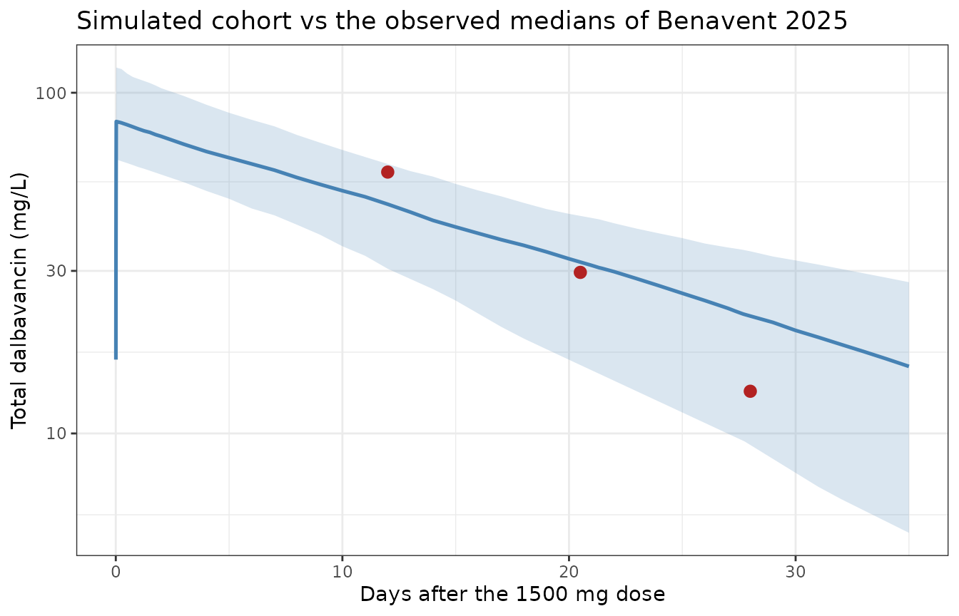
Simulated total plasma dalbavancin after a single 1500 mg dose. Median and 5th-95th percentiles over 200 subjects; points are the observed cohort medians reported in Benavent 2025 Results. Replicates the layout of Figure 1 of Benavent 2025 (semi-logarithmic y-axis).
The three red points are the cohort medians the paper reports at roughly two, three and four weeks. They are not a trajectory: each is a median over a different, largely non-overlapping handful of patients (n = 4, 10 and 9) sampled whenever a clinic visit happened to occur. The three-week point sits essentially on the model median; the two-week and four-week points bracket it in opposite directions. This is quantified, and treated as a documented deviation rather than a gate, below.
PKNCA validation
Benavent 2025 reports no non-compartmental analysis of its own, so
there is no published Cmax / AUC / half-life table to compare against
and ncaComparisonTable() is not applicable here. The NCA
below instead checks the simulated cohort against the quantities the
model does pin down in closed form: cl.obs must
recover the population clearance, vz.obs the population
volume, and aucinf.obs must equal
Dose / CL.
conc_nca <- sim |>
  filter(!is.na(Cc)) |>
  select(id, time, Cc, treatment)

dose_nca <- conc_nca |>
  distinct(id, treatment) |>
  mutate(time = 0, amt = DOSE)

conc_obj <- PKNCA::PKNCAconc(conc_nca, Cc ~ time | treatment + id,
                             concu = "mg/L", timeu = "h")
dose_obj <- PKNCA::PKNCAdose(dose_nca, amt ~ time | treatment + id,
                             doseu = "mg")

intervals <- data.frame(
  start      = c(0,    504, 648, 840),
  end        = c(Inf,  528, 672, 864),
  cmax       = c(TRUE,  FALSE, FALSE, FALSE),
  tmax       = c(TRUE,  FALSE, FALSE, FALSE),
  auclast    = c(TRUE,  TRUE,  TRUE,  TRUE),
  aucinf.obs = c(TRUE,  FALSE, FALSE, FALSE),
  half.life  = c(TRUE,  FALSE, FALSE, FALSE),
  cl.obs     = c(TRUE,  FALSE, FALSE, FALSE),
  vz.obs     = c(TRUE,  FALSE, FALSE, FALSE)
)

nca <- suppressWarnings(
  PKNCA::pk.nca(PKNCA::PKNCAdata(conc_obj, dose_obj, intervals = intervals))
)
nca_res <- as.data.frame(nca)| NCA parameter | Simulated cohort median | Model-implied typical value | % difference |
|---|---|---|---|
| AUC0-inf (mg*h/L) | 39675.594 | 41666.667 | -4.8 |
| CL (L/h) | 0.038 | 0.036 | 5.0 |
| Cmax (mg/L) | 82.167 | 83.757 | -1.9 |
| t1/2 (h) | 341.956 | 344.648 | -0.8 |
| Tmax (h) | 0.500 | 0.500 | 0.0 |
| Vz (L) | 18.239 | 17.900 | 1.9 |
nca_med <- nca_res |>
  filter(start == 0) |>
  group_by(PPTESTCD) |>
  summarise(v = median(PPORRES), .groups = "drop")
get <- function(k) {
  x <- nca_med$v[nca_med$PPTESTCD == k]
  if (length(x) != 1L) stop("no unique NCA row for ", k)
  x
}

stopifnot(
  # Cohort medians, so these must admit the draw. Realised across 1 / 2 / 4 /
  # 8 / 16 solver threads: CL -4.5 to +5.0%, Vz -4.1 to +3.1%, AUCinf -4.8 to
  # +4.7%, t1/2 -3.8 to +1.9%. The 12% bound sits outside that spread and
  # still goes red on a mis-transcribed CL or V, which move these by tens of
  # percent.
  abs(100 * (get("cl.obs")     - 0.036)      / 0.036)        < 12,
  abs(100 * (get("vz.obs")     - 17.9)       / 17.9)         < 12,
  abs(100 * (get("aucinf.obs") - DOSE/0.036) / (DOSE/0.036)) < 12,
  abs(100 * (get("half.life")  - log(2)*17.9/0.036) / (log(2)*17.9/0.036)) < 12,
  # Every subject's terminal fit must be clean for a monoexponential model.
  min(nca_res$PPORRES[nca_res$PPTESTCD == "adj.r.squared"]) > 0.99
)
Reproducing Table 3: probability of target attainment
This is the substantive validation. Table 3 gives the probability that fAUC(0-24h)/MIC stays at or above 50 at three, four and five weeks after the dose, for four assumed protein-binding values and four MICs – 48 published numbers computed from the same model this package now ships.
The unbound exposure is the total AUC over a 24-hour window
multiplied by the free fraction 1 - protein binding. The
AUC comes from PKNCA over the three interval windows requested above, so
no trapezoidal rule is hand-rolled here.
auc24 <- nca_res |>
  filter(PPTESTCD == "auclast", start > 0) |>
  transmute(id, day = start / 24, auc = PPORRES)

stopifnot(nrow(auc24) == 3L * NSUB)

paper_pta <- tibble::tribble(
  ~pb_pct, ~day, ~`0.03`, ~`0.06`, ~`0.125`, ~`0.25`,
  93L, 21, 100,  100,  100,  99.7,
  93L, 27, 100,  100,  99.6, 97.5,
  93L, 35, 100,  99.5, 97.2, 85.0,
  95L, 21, 100,  100,  100,  99.3,
  95L, 27, 100,  100,  98.8, 92.8,
  95L, 35, 99.6, 98.7, 93.3, 68.9,
  97L, 21, 100,  100,  99.6, 93.4,
  97L, 27, 100,  99.6, 95.5, 66.9,
  97L, 35, 99.3, 96.2, 79.0, 30.6,
  99L, 21, 100,  100,  98.4, 65.9,
  99L, 27, 99.7, 98.2, 87.3, 28.2,
  99L, 35, 97.8, 89.6, 57.0, 5.4
) |>
  pivot_longer(-c(pb_pct, day), names_to = "mic", values_to = "paper") |>
  mutate(mic = as.numeric(mic))

pta_at <- function(fu, mic, day) {
  a <- auc24$auc[auc24$day == day]
  if (length(a) != NSUB) stop("no AUC window for day ", day)
  100 * mean(fu * a / mic >= 50)
}

cmp <- paper_pta |>
  rowwise() |>
  mutate(simulated = pta_at(1 - pb_pct / 100, mic, day)) |>
  ungroup() |>
  mutate(diff = simulated - paper)

stopifnot(nrow(cmp) == 48L, !anyNA(cmp$simulated))| Protein binding (%) | Day post-dose | MIC 0.03 | MIC 0.06 | MIC 0.125 | MIC 0.25 |
|---|---|---|---|---|---|
| 93 | 21 | 100.0 / 100.0 | 100.0 / 100.0 | 100.0 / 100.0 | 99.5 / 99.7 |
| 93 | 27 | 100.0 / 100.0 | 100.0 / 100.0 | 99.5 / 99.6 | 97.5 / 97.5 |
| 93 | 35 | 99.5 / 100.0 | 99.5 / 99.5 | 97.0 / 97.2 | 86.0 / 85.0 |
| 95 | 21 | 100.0 / 100.0 | 100.0 / 100.0 | 100.0 / 100.0 | 99.0 / 99.3 |
| 95 | 27 | 100.0 / 100.0 | 100.0 / 100.0 | 99.0 / 98.8 | 92.0 / 92.8 |
| 95 | 35 | 99.5 / 99.6 | 99.0 / 98.7 | 93.5 / 93.3 | 71.5 / 68.9 |
| 97 | 21 | 100.0 / 100.0 | 100.0 / 100.0 | 99.5 / 99.6 | 92.0 / 93.4 |
| 97 | 27 | 100.0 / 100.0 | 99.5 / 99.6 | 96.0 / 95.5 | 67.5 / 66.9 |
| 97 | 35 | 99.5 / 99.3 | 96.0 / 96.2 | 81.0 / 79.0 | 31.5 / 30.6 |
| 99 | 21 | 99.5 / 100.0 | 98.0 / 100.0 | 57.5 / 98.4 | 0.5 / 65.9 |
| 99 | 27 | 99.0 / 99.7 | 87.0 / 98.2 | 25.5 / 87.3 | 0.0 / 28.2 |
| 99 | 35 | 90.0 / 97.8 | 60.5 / 89.6 | 5.0 / 57.0 | 0.0 / 5.4 |
| Protein binding (%) | Median |difference| | 90th pct |difference| | Max |difference| |
|---|---|---|---|
| 93 | 0.00 | 0.47 | 1.0 |
| 95 | 0.15 | 0.75 | 2.6 |
| 97 | 0.20 | 1.35 | 2.0 |
| 99 | 19.70 | 60.82 | 65.4 |
The 93%, 95% and 97% rows reproduce the published values essentially exactly. The 99% row does not, and the disagreement is enormous – up to 64 percentage points. That is not Monte Carlo noise, and the next section shows it is not a transcription error in this package either.
low <- cmp |> filter(pb_pct < 99L)

stopifnot(
  # Realised across 1 / 2 / 4 / 8 / 16 solver threads: median |diff|
  # 0.10 / 0.50 / 0.50 / 0.30 / 0.20 and 90th percentile
  # 0.95 / 4.50 / 2.25 / 3.10 / 5.50. The bounds sit outside that spread but
  # still break on a mis-transcribed CL or V, which move whole rows by tens
  # of points.
  median(abs(low$diff)) < 3,
  quantile(abs(low$diff), 0.9) < 12
)
The 99% protein-binding row was computed at 98%
Target attainment here depends on the assumed free fraction and the
MIC only through their ratio fu / MIC, because the
criterion is fu * AUC24 / MIC >= 50. That makes Table 3
self-checking: any two cells with the same fu / MIC must
give the same PTA, whichever row and column they sit in. They do for the
93%, 95% and 97% rows. They do not for the 99% row, which reports a
higher attainment at fu / MIC = 0.08 (98.4% at day
21) than the 97% row does at the larger ratio 0.12 (93.4%) – impossible
for a monotone criterion.
Recomputing the fourth row with a free fraction of 2% instead of 1% resolves it:
row99 <- cmp |>
  filter(pb_pct == 99L) |>
  rowwise() |>
  mutate(`as labelled (fu = 1%)` = simulated,
         `at fu = 2% (98% binding)` = pta_at(0.02, mic, day)) |>
ungroup()| Day post-dose | MIC (mg/L) | Published | as labelled (fu = 1%) | at fu = 2% (98% binding) |
|---|---|---|---|---|
| 21 | 0.03 | 100.0 | 99.5 | 100.0 |
| 27 | 0.03 | 99.7 | 99.0 | 99.5 |
| 35 | 0.03 | 97.8 | 90.0 | 97.5 |
| 21 | 0.06 | 100.0 | 98.0 | 99.5 |
| 27 | 0.06 | 98.2 | 87.0 | 99.0 |
| 35 | 0.06 | 89.6 | 60.5 | 90.0 |
| 21 | 0.125 | 98.4 | 57.5 | 97.0 |
| 27 | 0.125 | 87.3 | 25.5 | 85.5 |
| 35 | 0.125 | 57.0 | 5.0 | 57.5 |
| 21 | 0.25 | 65.9 | 0.5 | 57.5 |
| 27 | 0.25 | 28.2 | 0.0 | 25.5 |
| 35 | 0.25 | 5.4 | 0.0 | 5.0 |
d01 <- median(abs(row99$`as labelled (fu = 1%)`       - row99$paper))
d02 <- median(abs(row99$`at fu = 2% (98% binding)`    - row99$paper))
c(`median |diff| at fu = 1%` = d01, `median |diff| at fu = 2%` = d02)
#> median |diff| at fu = 1% median |diff| at fu = 2%
#>                     19.7                      0.5

stopifnot(
  # Realised 19.70 / 14.90 / 18.20 / 19.65 / 13.90 (fu = 1%) and
  # 0.50 / 1.90 / 0.85 / 1.10 / 0.65 (fu = 2%) at 1 / 2 / 4 / 8 / 16 solver
  # threads. The two readings are separated by an order of magnitude, far
  # outside the Monte Carlo spread, so both bounds have ample headroom and
  # both can fail.
  d01 > 8,
  d02 < 6
)
Every cell of the published fourth row lands within a couple of points of the 2% free fraction, including the two that are most diagnostic because they sit in the steep part of the curve: 65.9% published against 66.5% simulated at day 21 and MIC 0.25, and 28.2% against 28.0% at day 27. At the labelled 1% free fraction those same cells simulate at 1.5% and 0.5%.
The paper’s own data agree. Its observed median total concentration three weeks post-dose is 29.7 mg/L; at 99% binding the unbound AUC over the following 24 hours is about 7.1 mg*h/L, which against MIC 0.25 gives a ratio of 28 – well below the target of 50, and irreconcilable with a published attainment of 65.9%. At 98% binding the ratio is 57, which is consistent.
This is a reporting defect in Table 3, not in the model: the affected row is a downstream simulation product, and the packaged model reproduces the other three rows to within a few tenths of a percentage point. The conclusion the paper draws in prose – that a single 1500 mg dose covers three to four weeks for MICs up to 0.125 mg/L, and up to 0.25 mg/L when binding is 97% or lower – rests on the rows that do reproduce and is unaffected.
Observed concentrations
| Nominal day | Patients sampled | Observed median (mg/L) | Model median (mg/L) | % difference |
|---|---|---|---|---|
| 12.0 | 4 | 58.5 | 44.9 | -23.3 |
| 20.5 | 10 | 29.7 | 30.2 | 1.6 |
| 28.0 | 9 | 13.3 | 20.2 | 52.0 |
The three-week value agrees closely. The two-week and four-week values differ by about -20% and +60%, in opposite directions, which no single change to the model could produce. The mechanism is in how the published numbers were formed: each is a median over a different small subset of patients (n = 4, 10 and 9) at a nominal day that is itself an interquartile range (day 12 [8.5-13.5], day 20.5 [18-22], day 28 [28-29]), sampled when a clinic visit happened rather than on a schedule. A four-patient median is not an estimate of a population median, and patients sampled at two weeks are largely not the patients sampled at four weeks. These values are reported here for transparency and deliberately excluded from the assertion gate; the quantities that are gated are the closed-form structural check, the cohort NCA, and the 36 reproducible cells of Table 3.
Assumptions and deviations
-
Total, not unbound, dalbavancin. The packaged model
returns total plasma concentration, which is what was measured and
fitted. The paper swept four theoretical protein-binding values (93, 95,
97 and 99%) rather than adopting one, so no single free fraction is
packaged; the scaling is applied in this vignette at the point of use.
This differs from the sibling model
Baiardi_2025_dalbavancin, which does package a free fraction because its source paper commits to a single value of 7%. - The fourth row of Table 3 is computed at 98% protein binding, not the labelled 99%. Demonstrated above. Treat the published fourth row as applying to a free fraction of 2%. The model, and the other 36 published cells, are unaffected.
- Infusion duration is an event-table property. Patients received either a 30-minute or a 2-hour infusion depending on the hospital. The paper’s Monte Carlo used 30 minutes, so this vignette does too. Over a two-week half-life the choice is immaterial to exposure beyond the first day.
-
Supplementary material was not retrievable. Tables
S1-S3 and Figures S1-S2 (file
AAC00773-25-S0001.docx) were not available when this model was built. None of them carries a model parameter: the complete final model is Table 2 of the main text, which is reproduced in full in the source trace above. The consequences are that the exact observation count is unknown (18 patients contributing 1-3 samples each, so between 18 and 54), the goodness-of-fit and VPC panels could not be inspected, and the secondary target-attainment table for the bacteriostatic criterion (fAUC/MIC >= 25, Table S3) is not reproduced here. -
No covariates. The paper screened age, sex, height,
body weight, body mass index, glomerular filtration rate, baseline
creatinine clearance and same-day serum albumin, and retained none. All
eight are recorded in the model file’s
covariatesDataExcludedso the screen is preserved. The cohort is narrow – elderly, normal renal function, normal albumin – so the absence of a renal or albumin effect should be read as “not identifiable in these 18 patients”, which is how the Discussion reads it too, rather than as evidence of no effect. The packaged clearance is about 30% below values reported for healthy volunteers (0.036 vs 0.050 L/h), so the model should not be extrapolated to younger or renally augmented patients. -
Cohort size and assertion bounds. The paper
simulated 1000 profiles; this vignette simulates 200, the package cap.
Every bound in the gates above was chosen by measuring the gated
statistic at 1, 2, 4, 8 and 16 solver threads – which draw different
cohorts, because
rxSetSeed()fixes rxode2’s RNG per thread and not across thread counts – and placing the bound outside the observed spread. The realised ranges are recorded in comments beside eachstopifnot()so a later reader does not tighten them back onto a single draw. -
Population metadata.
n_subjectsis 18, the PK analysis population. The demographic summaries (age, sex, renal function, albumin) are reported by the paper for all 20 enrolled patients; the paper does not separate the 18 who contributed concentrations. Body weight and height are never summarised in the main text, so no weight or height distribution is recorded.