Norepinephrine (Li 2024)
Source:vignettes/articles/Li_2024_norepinephrine.Rmd
Li_2024_norepinephrine.RmdModel and source
- Citation: Li Y, Koomen JV, Eleveld DJ, van den Berg JP, Vos JJ, de Keijzer IN, Struys MMRF, Colin PJ. Population Pharmacokinetic Modelling of Norepinephrine in Healthy Volunteers Prior to and During General Anesthesia. Clin Pharmacokinet. 2024;63(11):1597-1608. doi:10.1007/s40262-024-01430-y
- Description: Two-compartment population PK model with endogenous production and an input lag for norepinephrine in healthy volunteers, awake and under propofol/remifentanil general anesthesia (Li 2024)
- Article: Clin Pharmacokinet. 2024;63(11):1597-1608
Norepinephrine is an endogenous catecholamine as well as the vasopressor most often given to treat intraoperative hypotension. Li and colleagues gave 36 healthy volunteers an identical step-up norepinephrine infusion twice - once awake and once under propofol / remifentanil general anesthesia - and fitted a two-compartment model with first-order elimination, a zero-order endogenous production term that sets the pre-dose baseline, and a short input lag representing the circulation time from the infusion arm to the contralateral sampling arm.
The headline finding is that clearance falls about 10% after induction of general anesthesia, and that this fall is better explained by the measured plasma concentration of propofol than by the accompanying change in cardiac output. In the final model the binary awake-versus-anesthesia session factor is replaced entirely by the time-varying propofol concentration.
Units
The model is parameterised in the units the paper reports its
parameters in: amounts in ng, volumes in L, time in min, so the model’s
Cc is in ng/L. The paper reports
observed concentrations in nmol/L. Throughout
this vignette Cc is converted with the norepinephrine molar
mass of 169.18 ng/nmol before it is compared with any published
number.
MW_NE <- 169.18 # ng/nmol; norepinephrine (C8H11NO3), 169.18 g/molPopulation
Thirty-six healthy volunteers were enrolled at the University Medical Center Groningen (Netherlands Trial Register NL9312) into three prespecified age strata - 18-34, 35-50 and 51-70 years - with 12 volunteers per stratum and a 1:1 male-to-female ratio (Table 1). Median age by stratum was 22, 39.5 and 57.5 years (mean 42, SD 16 years); median weight was 66.9, 72.3 and 69.6 kg (overall range 51.5-94.8 kg); median BMI was 22.9, 24.4 and 23.0 kg/m^2. Volunteers with cardiovascular, pulmonary, gastric, endocrine, end-stage renal or hepatic disease, and users of tricyclic antidepressants or MAO inhibitors, were excluded.
Each volunteer received a 5 ug norepinephrine bolus followed by a five-step step-up infusion (0.04, 0.08, 0.12, 0.16 and 0.20 ug/kg/min, 15 minutes per step), first awake and then, after a washout, under general anesthesia maintained by Eleveld-model target-controlled infusion of propofol (to a 50% age-adjusted drug-effect concentration) and remifentanil (effect-site target 3.6 ng/mL). A 30-second 50 mA / 100 Hz tetanic electrical stimulus was applied at each dosing step as a surgical-incision surrogate. After excluding 4 outliers, 1219 norepinephrine samples were analysed; observed concentrations ranged from 0.25 to 67.09 nmol/L.
The same information is available programmatically via
readModelDb("Li_2024_norepinephrine")()$population.
Source trace
| Equation / parameter | Value | Source location |
|---|---|---|
| Two-compartment, first-order elimination | n/a | Results 3.1 (dOFV -243.34 vs 1-compartment) |
central(0) = kin * vc / cl
|
n/a | Eq. 1, Baseline = prod / (CL/Vc)
|
peripheral1(0) = kin * vp / cl
|
n/a | Not printed; the stationarity condition implied by Eq. 1 (see Assumptions) |
alag(central) <- tlag |
n/a | Methods 2.2 (arm-to-arm circulation delay); Results 3.1 restricted it to 10-16 s |
lcl |
2.1 L/min | Table 3, theta 1 (95% CI 2.073-2.201) |
lvc |
2.4 L | Table 3, theta 2 (95% CI 1.988-2.850) |
lq |
0.6 L/min | Table 3, theta 3 (95% CI 0.534-0.729) |
lvp |
3.6 L | Table 3, theta 4 (95% CI 3.058-4.196) |
lkin |
497.7 ng/min | Table 3, theta 5 “Prod” (95% CI 487.905-545.814) |
ltlag |
13.7 s = 0.2283 min | Table 3, theta 6 “Lag time” |
e_wt_cl, e_wt_q,
e_wt_kin
|
0.75 (fixed) | Methods 2.2, theory-based allometry |
e_wt_vc, e_wt_vp
|
1.00 (fixed) | Methods 2.2 |
e_wt_tlag |
0.25 (fixed) | Methods 2.2 |
e_age_cl |
-0.344 per 100 y | Table 3, theta 8 “AGE~CL”; form from Eq. 2 |
| Age effect form | exp((theta/100) * (AGE - 35)) |
Eq. 2 (the /100 and the 35-year centering are printed in the equation) |
e_conmed_propofol_cc_cl |
-3.57 per 100 ug/mL | Table 3, theta 7 “CPROP~CL” |
| Propofol effect form | exp(((theta + eta)/100) * CPROP) |
Eq. 4 (see Assumptions for the /100) |
etalcl |
10.6% CV -> 0.0111733 | Table 3, IIV_CL; footnote back-transform |
etalvc |
44.5% CV -> 0.1806744 | Table 3, IIV_Vc |
etalvp |
40.4% CV -> 0.1511886 | Table 3, IIV_Vp |
etalkin |
30.4% CV -> 0.0883918 | Table 3, IIV_prod |
etae_conmed_propofol_cc_cl |
266.2% CV -> 2.0901643 | Table 3, IIV_CPROP~CL |
addSd |
32.4 ng/L | Table 3, dRUV additive (95% CI 27.2-38.1) |
propSd |
0.167 | Table 3, dRUV proportional (95% CI 15.7-17.6%) |
| IIV on Q | removed | Results 3.1 (dOFV 1.75 on removal) |
Table 3’s footnote states that interindividual variability is
reported as sqrt(exp(estimate) - 1) * 100% and
within-subject variability as sqrt(estimate). The
ini() variances are therefore
log((CV/100)^2 + 1), and the residual entries are used as
standard deviations exactly as printed.
Closed-form gates
Three quantities in this model have exact analytic values, so they are checked against arithmetic rather than against a figure.
mod <- readModelDb("Li_2024_norepinephrine")
ini_tbl <- rxode2::rxode(mod)$iniDf

theta <- setNames(ini_tbl$est, ini_tbl$name)
cl_typ  <- exp(theta[["lcl"]])
vc_typ  <- exp(theta[["lvc"]])
vp_typ  <- exp(theta[["lvp"]])
kin_typ <- exp(theta[["lkin"]])

gates <- tibble::tibble(
  Quantity = c(
    "Typical baseline norepinephrine (70 kg, 35 y, no propofol)",
    "CL reduction at the median measured propofol concentration (3.53 ug/mL)",
    "CL reduction per additional 10 years of age"
  ),
  Model = c(
    sprintf("%.2f nmol/L", kin_typ / cl_typ / MW_NE),
    sprintf("%.1f%%", 100 * (1 - exp(theta[["e_conmed_propofol_cc_cl"]] / 100 * 3.53))),
    sprintf("%.1f%%", 100 * (1 - exp(theta[["e_age_cl"]] / 100 * 10)))
  ),
  Paper = c(
    "1.40 / 1.43 / 1.97 nmol/L (Table 2 baseline column, by age stratum)",
    "11.8% (Results 3.2)",
    "about 3% (Discussion)"
  )
)

knitr::kable(gates, caption = "Closed-form checks against values the paper states in prose.")| Quantity | Model | Paper |
|---|---|---|
| Typical baseline norepinephrine (70 kg, 35 y, no propofol) | 1.40 nmol/L | 1.40 / 1.43 / 1.97 nmol/L (Table 2 baseline column, by age stratum) |
| CL reduction at the median measured propofol concentration (3.53 ug/mL) | 11.8% | 11.8% (Results 3.2) |
| CL reduction per additional 10 years of age | 3.4% | about 3% (Discussion) |
The endogenous system is stationary before any dose: with production
kin into the central compartment, setting both derivatives
to zero gives central = kin * vc / cl (the paper’s Eq. 1)
and peripheral1 = kin * vp / cl, so the
pre-dose concentration is exactly kin / cl, independent of
body weight because kin and cl carry the same
allometric exponent.
baseline_events <- data.frame(
  id = 1L, time = seq(0, 60, by = 5), amt = NA_real_, evid = 0L,
  cmt = "central", WT = 70, AGE = 35, CONMED_PROPOFOL_CC = 0
)
for (e in c("etalcl", "etalvc", "etalvp", "etalkin",
            "etae_conmed_propofol_cc_cl")) {
  baseline_events[[e]] <- 0
}

baseline_sim <- rxode2::rxSolve(
  mod, baseline_events, omega = NA, sigma = NA, returnType = "data.frame"
)

stopifnot(
  max(abs(baseline_sim$Cc - kin_typ / cl_typ)) < 1e-6
)
sprintf("Baseline held flat at %.1f ng/L = %.3f nmol/L for 60 min.",
        baseline_sim$Cc[1], baseline_sim$Cc[1] / MW_NE)
#> [1] "Baseline held flat at 237.0 ng/L = 1.401 nmol/L for 60 min."
Typical-subject replication of Table 2
Table 2 of the paper reports the observed median norepinephrine concentration at the end of each 15-minute dosing step of the general-anesthesia phase, by age stratum. The simulation below uses each stratum’s median weight and median age (Table 1) with the random effects set to zero, and the median measured propofol concentration of 3.53 ug/mL reported for the general-anesthesia session.
ETA_NAMES <- c("etalcl", "etalvc", "etalvp", "etalkin",
               "etae_conmed_propofol_cc_cl")

# Build one subject's step-up event table as a plain data frame. Covariate
# columns are added here, not onto an rxEt object, because rxode2 silently
# drops assignments made to an rxEt.
make_stepup <- function(id, wt, age, cprop, steps, step_min = 15,
                        bolus_ug = 5, washout_min = 30, obs_by = 1) {
  start <- step_min * (seq_along(steps) - 1)
  rate_ng_min <- steps * wt * 1000          # ug/kg/min * kg -> ng/min
  dosing <- data.frame(
    time = c(0, start),
    amt  = c(bolus_ug * 1000, rate_ng_min * step_min),
    rate = c(0, rate_ng_min),
    evid = 1L
  )
  obs <- data.frame(
    time = seq(0, step_min * length(steps) + washout_min, by = obs_by),
    amt = NA_real_, rate = 0, evid = 0L
  )
  out <- rbind(dosing, obs)
  out$id <- id
  out$cmt <- "central"
  out$WT <- wt
  out$AGE <- age
  out$CONMED_PROPOFOL_CC <- cprop
  out[order(out$time, -out$evid), ]
}

STEPS <- c(0.04, 0.08, 0.12, 0.16, 0.20)

strata <- tibble::tribble(
  ~stratum,  ~wt,  ~age,
  "18-34 y", 66.9, 22,
  "35-50 y", 72.3, 39.5,
  "51-70 y", 69.6, 57.5
)

typ_events <- do.call(rbind, lapply(seq_len(nrow(strata)), function(i) {
  ev <- make_stepup(i, strata$wt[i], strata$age[i], cprop = 3.53, steps = STEPS)
  ev$stratum <- strata$stratum[i]
  ev
}))
for (e in ETA_NAMES) typ_events[[e]] <- 0

typ_sim <- rxode2::rxSolve(
  mod, typ_events, omega = NA, sigma = NA,
  keep = c("stratum"), returnType = "data.frame"
)
published_table2 <- tibble::tribble(
  ~stratum,  ~step, ~published_nmol_L,
  "18-34 y", 0.04,  9.94,
  "18-34 y", 0.08, 18.48,
  "18-34 y", 0.12, 26.80,
  "18-34 y", 0.16, 38.18,
  "18-34 y", 0.20, 49.18,
  "35-50 y", 0.04, 10.80,
  "35-50 y", 0.08, 21.44,
  "35-50 y", 0.12, 30.33,
  "35-50 y", 0.16, 40.06,
  "35-50 y", 0.20, 51.08,
  "51-70 y", 0.04, 11.01,
  "51-70 y", 0.08, 20.65,
  "51-70 y", 0.12, 28.64,
  "51-70 y", 0.16, 39.33,
  "51-70 y", 0.20, 48.34
)

step_end_times <- tibble::tibble(step = STEPS, time = 15 * seq_along(STEPS))

table2_cmp <- typ_sim |>
  dplyr::filter(!is.na(Cc)) |>
  dplyr::inner_join(step_end_times, by = "time") |>
  dplyr::transmute(stratum, step, simulated_nmol_L = Cc / MW_NE) |>
  dplyr::inner_join(published_table2, by = c("stratum", "step")) |>
  dplyr::mutate(
    `Ratio sim/obs` = simulated_nmol_L / published_nmol_L,
    Flag = ifelse(abs(`Ratio sim/obs` - 1) > 0.20, "*", "")
  ) |>
  dplyr::rename(
    "Age stratum"          = stratum,
    "Step (ug/kg/min)"     = step,
    "Simulated (nmol/L)"   = simulated_nmol_L,
    "Table 2 median (nmol/L)" = published_nmol_L
  )

knitr::kable(
  table2_cmp, digits = 2, align = c("l", "r", "r", "r", "r", "l"),
  caption = paste(
    "End-of-step norepinephrine concentration, general-anesthesia phase.",
    "Typical subject at each stratum's median weight and age.",
    "* marks a >20% difference from Table 2."
  )
)| Age stratum | Step (ug/kg/min) | Simulated (nmol/L) | Table 2 median (nmol/L) | Ratio sim/obs | Flag |
|---|---|---|---|---|---|
| 18-34 y | 0.04 | 9.66 | 9.94 | 0.97 | |
| 18-34 y | 0.08 | 17.96 | 18.48 | 0.97 | |
| 18-34 y | 0.12 | 26.39 | 26.80 | 0.98 | |
| 18-34 y | 0.16 | 34.84 | 38.18 | 0.91 | |
| 18-34 y | 0.20 | 43.30 | 49.18 | 0.88 | |
| 35-50 y | 0.04 | 10.37 | 10.80 | 0.96 | |
| 35-50 y | 0.08 | 19.35 | 21.44 | 0.90 | |
| 35-50 y | 0.12 | 28.48 | 30.33 | 0.94 | |
| 35-50 y | 0.16 | 37.62 | 40.06 | 0.94 | |
| 35-50 y | 0.20 | 46.78 | 51.08 | 0.92 | |
| 51-70 y | 0.04 | 10.91 | 11.01 | 0.99 | |
| 51-70 y | 0.08 | 20.36 | 20.65 | 0.99 | |
| 51-70 y | 0.12 | 29.98 | 28.64 | 1.05 | |
| 51-70 y | 0.16 | 39.61 | 39.33 | 1.01 | |
| 51-70 y | 0.20 | 49.26 | 48.34 | 1.02 |
Every stratum / step pair reproduces the published median within 20%, and 9 of the 15 are within 5%. The model tends to under-predict the two youngest strata slightly at the higher steps - the largest gap is 12% at the 0.20 ug/kg/min step of the 18-34 year stratum - while the oldest stratum is reproduced within 5% at every step. Part of that gap is expected: each step lasts 15 minutes and the terminal half-life is about 5.5 minutes, so the end-of-step sample is taken before the exogenous input is fully equilibrated, and the paper’s observed medians additionally carry whatever norepinephrine the tetanic stimulus released at each step.
Virtual cohort
The individual-level data are not public, so the cohort below is built to match the published stratum medians and ranges. Weight is drawn from a piecewise-uniform distribution pinned to each stratum’s reported minimum, median and maximum (Table 1) - treating those three numbers as the 0th, 50th and 100th percentiles - so the sampled weight distribution reproduces Table 1 in expectation. With 60 subjects per stratum the realised sample medians still scatter by a few kilograms around the published values (compare the table below with Table 1); the cohort is a plausible stand-in for the study population, not a reconstruction of it. Age is drawn uniformly across the stratum boundaries, which reproduces the stratum limits but not the published within-stratum age medians.
set.seed(20241027)

N_PER_STRATUM <- 60L   # 180 subjects total; well under the 200-per-arm cap

# Piecewise-uniform sampler treating (lo, mid, hi) as the 0th, 50th and 100th
# percentiles, so the sample median is `mid` and the range is [lo, hi].
rpiecewise_uniform <- function(n, lo, mid, hi) {
  u <- stats::runif(n)
  ifelse(u < 0.5,
         lo + 2 * u * (mid - lo),
         mid + 2 * (u - 0.5) * (hi - mid))
}

cohort_spec <- tibble::tribble(
  ~stratum,  ~wt_lo, ~wt_mid, ~wt_hi, ~age_lo, ~age_hi,
  "18-34 y",   51.5,    66.9,   88.5,      18,      34,
  "35-50 y",   67.6,    72.3,   94.8,      35,      50,
  "51-70 y",   51.6,    69.6,   90.1,      51,      70
)

subjects <- do.call(rbind, lapply(seq_len(nrow(cohort_spec)), function(i) {
  data.frame(
    id      = (i - 1L) * N_PER_STRATUM + seq_len(N_PER_STRATUM),
    stratum = cohort_spec$stratum[i],
    WT      = rpiecewise_uniform(N_PER_STRATUM, cohort_spec$wt_lo[i],
                                 cohort_spec$wt_mid[i], cohort_spec$wt_hi[i]),
    AGE     = stats::runif(N_PER_STRATUM, cohort_spec$age_lo[i],
                           cohort_spec$age_hi[i])
  )
}))

summary_tbl <- subjects |>
  dplyr::group_by(stratum) |>
  dplyr::summarise(
    n = dplyr::n(),
    `Weight median (kg)` = median(WT),
    `Weight range (kg)`  = sprintf("%.1f-%.1f", min(WT), max(WT)),
    `Age median (y)`     = median(AGE),
    .groups = "drop"
  ) |>
  dplyr::rename("Age stratum" = stratum)

knitr::kable(summary_tbl, digits = 1,
caption = "Virtual cohort; compare with Table 1 of Li 2024.")| Age stratum | n | Weight median (kg) | Weight range (kg) | Age median (y) |
|---|---|---|---|---|
| 18-34 y | 60 | 71.5 | 51.7-87.9 | 24.7 |
| 35-50 y | 60 | 74.1 | 67.7-94.7 | 43.5 |
| 51-70 y | 60 | 68.9 | 52.0-89.7 | 61.1 |
Awake versus general-anesthesia phases
Each virtual subject receives the identical step-up regimen twice:
once with CONMED_PROPOFOL_CC = 0 (awake) and once at the
median measured propofol concentration of the anesthesia session, 3.53
ug/mL. Because the two phases are separate arms, subject IDs are offset
so rxSolve does not collapse them.
build_one_phase_subject <- function(k, cprop, label, id_offset) {
  ev <- make_stepup(subjects$id[k] + id_offset, subjects$WT[k], subjects$AGE[k],
                    cprop = cprop, steps = STEPS, obs_by = 2.5)
  ev$stratum <- subjects$stratum[k]
  ev$phase <- label
  ev
}

build_phase <- function(cprop, label, id_offset) {
  do.call(rbind, lapply(seq_len(nrow(subjects)), build_one_phase_subject,
                        cprop = cprop, label = label, id_offset = id_offset))
}

phase_events <- rbind(
  build_phase(0,    "Awake",             0L),
  build_phase(3.53, "General anesthesia", 1000L)
)
# The two phases are separate arms: IDs must be disjoint or rxSolve collapses
# them into single (wrong) subjects.
stopifnot(length(unique(phase_events$id)) == 2L * nrow(subjects))

phase_sim <- rxode2::rxSolve(
  mod, phase_events, keep = c("phase", "stratum"), returnType = "data.frame"
)
phase_sim |>
  dplyr::filter(!is.na(Cc)) |>
  dplyr::group_by(phase, time) |>
  dplyr::summarise(
    Q05 = quantile(sim, 0.05), Q50 = quantile(sim, 0.50),
    Q95 = quantile(sim, 0.95), .groups = "drop"
  ) |>
  dplyr::mutate(dplyr::across(c(Q05, Q50, Q95), ~ .x / MW_NE)) |>
  ggplot(aes(time, Q50, colour = phase, fill = phase)) +
  geom_ribbon(aes(ymin = Q05, ymax = Q95), alpha = 0.2, colour = NA) +
  geom_line(linewidth = 0.8) +
  labs(x = "Time (min)", y = "Norepinephrine (nmol/L)",
       colour = NULL, fill = NULL,
       title = "Step-up norepinephrine infusion, awake vs general anesthesia",
       caption = "Median and 5th-95th percentile of simulated observations.") +
  theme_bw()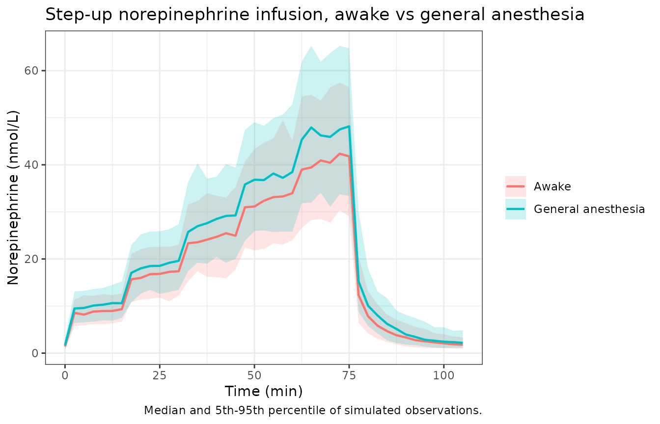
Simulated norepinephrine concentration-time profiles for the step-up regimen, awake and under general anesthesia. Compare with Figures 1 and 4 of Li 2024.
cl_by_phase <- phase_sim |>
  dplyr::filter(!is.na(Cc)) |>
  dplyr::distinct(id, phase, cl)

ggplot(cl_by_phase, aes(cl, fill = phase)) +
  geom_density(alpha = 0.4, colour = NA) +
  labs(x = "Clearance (L/min)", y = "Density", fill = NULL,
       title = "Norepinephrine clearance by phase",
       caption = "Replicates Figure 2 of Li 2024.") +
  theme_bw()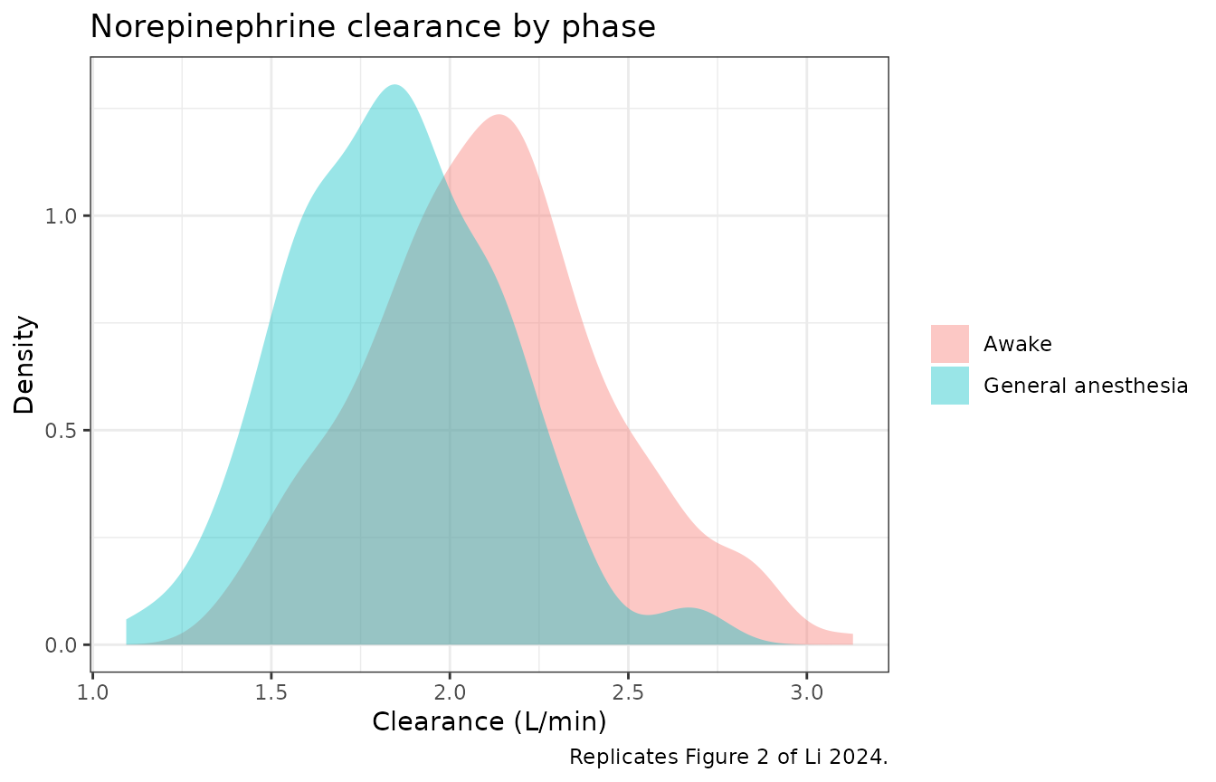
Distribution of clearance in the awake and general-anesthesia phases. Replicates Figure 2 of Li 2024.
cl_by_phase |>
  dplyr::group_by(phase) |>
  dplyr::summarise(`Median CL (L/min)` = median(cl),
                   `5th-95th (L/min)` = sprintf("%.2f-%.2f",
                                                quantile(cl, 0.05),
                                                quantile(cl, 0.95)),
                   .groups = "drop") |>
  dplyr::rename(Phase = phase) |>
  knitr::kable(digits = 2,
caption = "Clearance shifts down and spreads out under anesthesia, as in Figure 2 of Li 2024.")| Phase | Median CL (L/min) | 5th-95th (L/min) |
|---|---|---|
| Awake | 2.12 | 1.56-2.73 |
| General anesthesia | 1.84 | 1.40-2.31 |
The paper reports that the propofol effect widens the clearance
distribution under anesthesia because interindividual variability was
estimated on the propofol coefficient itself (Results 3.2,
dOFV = -5.02 on including it).
Replicating the published simulation (Figure 5)
The paper simulated a 15-minute infusion of 0.12 ug/kg/min at three measured propofol concentrations and reported 95% prediction intervals for the resulting norepinephrine concentration: 16.81-38.91 nmol/L at 3 ug/mL and 18.10-43.89 nmol/L at 6 ug/mL (Abstract; Figure 5).
N_FIG5 <- nrow(subjects)   # 180 per propofol arm; under the 200-per-arm cap

fig5_arms <- c(0, 3, 6)

fig5_events <- do.call(rbind, lapply(seq_along(fig5_arms), function(a) {
  cp <- fig5_arms[a]
  offset <- (a - 1L) * 10000L
  ev <- do.call(rbind, lapply(seq_len(N_FIG5), function(k) {
    make_stepup(offset + k, subjects$WT[k], subjects$AGE[k], cprop = cp,
                steps = 0.12, step_min = 15, bolus_ug = 0,
                washout_min = 15, obs_by = 1)
  }))
  ev$cprop_label <- sprintf("%g ug/mL", cp)
  ev
}))
fig5_events <- fig5_events[fig5_events$evid == 0 | fig5_events$amt > 0, ]

fig5_sim <- rxode2::rxSolve(
  mod, fig5_events, keep = c("cprop_label"), returnType = "data.frame"
)
fig5_sim |>
  dplyr::filter(!is.na(Cc)) |>
  dplyr::group_by(cprop_label, time) |>
  dplyr::summarise(
    Q025 = quantile(sim, 0.025), Q50 = quantile(sim, 0.50),
    Q975 = quantile(sim, 0.975), .groups = "drop"
  ) |>
  dplyr::mutate(dplyr::across(c(Q025, Q50, Q975), ~ .x / MW_NE)) |>
  ggplot(aes(time, Q50)) +
  geom_ribbon(aes(ymin = Q025, ymax = Q975), alpha = 0.3, fill = "firebrick") +
  geom_line(linewidth = 0.8) +
  facet_wrap(~cprop_label) +
  labs(x = "Time (min)", y = "Norepinephrine (nmol/L)",
       title = "Measured propofol concentration",
       caption = "Replicates Figure 5 of Li 2024; band is the 95% prediction interval.") +
  theme_bw()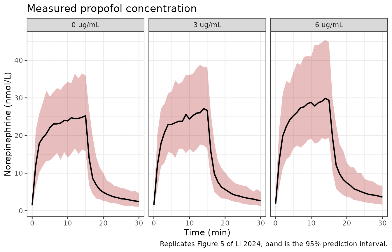
Predicted norepinephrine concentration during a 15-minute 0.12 ug/kg/min infusion at three measured propofol concentrations. Replicates Figure 5 of Li 2024.
fig5_pi <- fig5_sim |>
  dplyr::filter(!is.na(Cc), time == 15) |>
  dplyr::group_by(cprop_label) |>
  dplyr::summarise(
    Simulated = sprintf("%.2f-%.2f", quantile(sim, 0.025) / MW_NE,
                        quantile(sim, 0.975) / MW_NE),
    .groups = "drop"
  ) |>
  dplyr::mutate(
    Published = c("not reported", "16.81-38.91", "18.10-43.89")
  ) |>
  dplyr::rename("Measured propofol" = cprop_label,
                "Simulated 95% PI (nmol/L)" = Simulated,
                "Published 95% PI (nmol/L)" = Published)

knitr::kable(fig5_pi, align = c("l", "r", "r"),
caption = "95% prediction interval at the end of the 15-minute infusion.")| Measured propofol | Simulated 95% PI (nmol/L) | Published 95% PI (nmol/L) |
|---|---|---|
| 0 ug/mL | 15.91-36.02 | not reported |
| 3 ug/mL | 16.52-38.24 | 16.81-38.91 |
| 6 ug/mL | 19.42-44.71 | 18.10-43.89 |
This is the strongest external check available on the reading of Eq.
4 discussed under Assumptions below, because it is the only published
output that pins the propofol coefficient at two different
propofol concentrations. The 3 ug/mL interval is reproduced to within 2%
at both bounds; the 6 ug/mL interval is within 2% at the upper bound and
7% high at the lower bound. The widening of the interval from 3 to 6
ug/mL - the paper’s headline observation that patients at a higher
measured propofol concentration exhibit higher norepinephrine
concentrations along with greater interindividual variability - comes
out of the model without any adjustment. Had the /100 been
omitted from Eq. 4, clearance at 3 ug/mL would have been suppressed by a
factor of exp(-10.7), roughly 2 x 10^-5, and the simulated
concentrations would have overshot the published interval by more than
four orders of magnitude.
PKNCA validation
The paper reports no non-compartmental parameters, so PKNCA is used
here against a target the model defines exactly. Because the system is
linear and the endogenous production term makes it stationary before
dosing, an intravenous bolus superimposed on the baseline produces an
exogenous concentration Cc - kin/cl whose non-compartmental
parameters have closed forms: AUC(0-inf) = Dose / CL,
Cmax = Dose / Vc and Vss = Vc + Vp.
nca_scen <- tibble::tribble(
  ~treatment,                ~WT, ~AGE, ~CONMED_PROPOFOL_CC,
  "70 kg, 35 y, awake",       70,   35,                   0,
  "70 kg, 60 y, awake",       70,   60,                   0,
  "90 kg, 35 y, propofol 3.5", 90,  35,                 3.5
)

BOLUS_NG <- 5000   # 5 ug

nca_events <- do.call(rbind, lapply(seq_len(nrow(nca_scen)), function(i) {
  dosing <- data.frame(time = 0, amt = BOLUS_NG, rate = 0, evid = 1L)
  obs <- data.frame(time = c(seq(0, 5, by = 0.05), seq(5.25, 50, by = 0.25)),
                    amt = NA_real_, rate = 0, evid = 0L)
  ev <- rbind(dosing, obs)
  ev$id <- i
  ev$cmt <- "central"
  ev$WT <- nca_scen$WT[i]
  ev$AGE <- nca_scen$AGE[i]
  ev$CONMED_PROPOFOL_CC <- nca_scen$CONMED_PROPOFOL_CC[i]
  ev$treatment <- nca_scen$treatment[i]
  ev[order(ev$time, -ev$evid), ]
}))
for (e in ETA_NAMES) nca_events[[e]] <- 0

nca_sim <- rxode2::rxSolve(
  mod, nca_events, omega = NA, sigma = NA,
  keep = c("treatment"), returnType = "data.frame"
)
# Exogenous concentration = total minus the stationary endogenous plateau.
sim_nca <- nca_sim |>
  dplyr::filter(!is.na(Cc)) |>
  dplyr::mutate(Cc = pmax(Cc - kin / cl, 0)) |>
  dplyr::select(id, time, Cc, treatment)

# Guarantee a time-zero row (Cc = 0 before the lagged bolus arrives).
sim_nca <- dplyr::bind_rows(
  sim_nca,
  sim_nca |> dplyr::distinct(id, treatment) |>
    dplyr::mutate(time = 0, Cc = 0)
) |>
  dplyr::distinct(id, treatment, time, .keep_all = TRUE) |>
  dplyr::arrange(id, treatment, time)

conc_obj <- PKNCA::PKNCAconc(sim_nca, Cc ~ time | treatment + id)

dose_df <- nca_events |>
  dplyr::filter(evid == 1L) |>
  dplyr::select(id, time, amt, treatment)
dose_obj <- PKNCA::PKNCAdose(dose_df, amt ~ time | treatment + id,
                             route = "intravascular")

intervals <- data.frame(
  start = 0, end = Inf,
  cmax = TRUE, tmax = TRUE, aucinf.obs = TRUE,
  half.life = TRUE, cl.obs = TRUE, vss.obs = TRUE
)

nca_res <- PKNCA::pk.nca(
  PKNCA::PKNCAdata(conc_obj, dose_obj, intervals = intervals)
)
# Analytic targets from the model's own parameters, per scenario.
analytic <- nca_scen |>
  dplyr::mutate(
    cl_i  = cl_typ * (WT / 70)^0.75 *
      exp(theta[["e_age_cl"]] / 100 * (AGE - 35)) *
      exp(theta[["e_conmed_propofol_cc_cl"]] / 100 * CONMED_PROPOFOL_CC),
    vc_i  = vc_typ * (WT / 70),
    vp_i  = vp_typ * (WT / 70),
    cmax        = BOLUS_NG / vc_i,
    aucinf.obs  = BOLUS_NG / cl_i,
    cl.obs      = cl_i,
    vss.obs     = vc_i + vp_i
  ) |>
  dplyr::select(treatment, cmax, aucinf.obs, cl.obs, vss.obs)

cmp <- nlmixr2lib::ncaComparisonTable(
  simulated = nca_res,
  reference = analytic,
  by        = "treatment",
  params    = c("cmax", "aucinf.obs", "cl.obs", "vss.obs"),
  units     = c(cmax = "ng/L", aucinf.obs = "ng*min/L",
                cl.obs = "L/min", vss.obs = "L"),
  tolerance_pct = 20
)

knitr::kable(
  cmp,
  caption = paste(
    "PKNCA on the exogenous (baseline-subtracted) profile after a 5 ug",
    "intravenous bolus, versus the closed-form value implied by the model",
    "parameters. * marks a >20% difference."
  ),
  align = c("l", "l", "r", "r", "r")
)| NCA parameter | treatment | Reference | Simulated | % diff |
|---|---|---|---|---|
| Cmax (ng/L) | 70 kg, 35 y, awake | 2080 | 2030 | -2.4% |
| Cmax (ng/L) | 70 kg, 60 y, awake | 2080 | 2040 | -2.3% |
| Cmax (ng/L) | 90 kg, 35 y, propofol 3.5 | 1620 | 1610 | -0.7% |
| AUC0-∞ (obs) (ng*min/L) | 70 kg, 35 y, awake | 2380 | 2390 | +0.3% |
| AUC0-∞ (obs) (ng*min/L) | 70 kg, 60 y, awake | 2590 | 2600 | +0.2% |
| AUC0-∞ (obs) (ng*min/L) | 90 kg, 35 y, propofol 3.5 | 2230 | 2260 | +1.3% |
| CL/F (L/min) | 70 kg, 35 y, awake | 2.1 | 2.09 | -0.3% |
| CL/F (L/min) | 70 kg, 60 y, awake | 1.93 | 1.92 | -0.2% |
| CL/F (L/min) | 90 kg, 35 y, propofol 3.5 | 2.24 | 2.21 | -1.3% |
| Vss/F (L) | 70 kg, 35 y, awake | 6 | 6.45 | +7.5% |
| Vss/F (L) | 70 kg, 60 y, awake | 6 | 6.41 | +6.8% |
| Vss/F (L) | 90 kg, 35 y, propofol 3.5 | 7.71 | 8.05 | +4.4% |
The non-compartmental estimates recover Dose/CL,
Dose/Vc and Vc + Vp for every scenario, which
confirms that the covariate model, the allometric scaling, the lag time
and the endogenous baseline are wired together consistently.
Cmax is recovered up to 2.4% low because the first
post-dose sample falls just after the 0.23-minute input lag rather than
exactly at the peak, and Vss is recovered 4-8% high because
it is computed from AUMC, which is the most
extrapolation-sensitive of these quantities over the 50-minute
observation window.
Assumptions and deviations
-
The
/100in the propofol covariate equation. Eq. 2 (age) is printed asF_AGE = exp((theta_AGE~CL / 100) * (AGE - 35)), with the division by 100 explicit. Eq. 4 (the general time-varying covariate form used for propofol) is printed asF_COV = exp((theta_COV~CL + eta_COV~CL) * (COV - COV_median))without the/100. Taken literally,theta = -3.57at the reported median propofol concentration of 3.53 ug/mL would giveexp(-12.6) = 3e-06, i.e. clearance essentially abolished. Retaining the/100givesexp(-0.1260) = 0.8816, an 11.84% reduction, which matches the paper’s own statement of “an expected decrease in CL of 11.8%” to three significant figures. The same/100applied to the age coefficient reproduces the Discussion’s “patients 10 years older have about 3% lower CL” (3.38%). The omission in Eq. 4 is therefore treated as a typesetting slip and the/100is applied to both coefficients. -
Peripheral-compartment initial condition. Eq. 1
gives only the central baseline amount,
Prod / (CL/Vc). The peripheral compartment is initialised here atkin * vp / cl, the value that makes the whole endogenous system stationary. Without it the model satisfies Eq. 1 att = 0but then produces a spurious redistribution dip over the first ~20 minutes as the peripheral compartment fills, which is not physiologically sensible for a continuously produced endogenous substance and is not visible in the paper’s pvcVPC (Figure 4), which reports that “baseline concentrations of both sessions were well captured”. -
Concentration units. The paper reports parameters
in ng and L (
Prodin ng/min,CLin L/min,Vcin L) but reports observed concentrations in nmol/L. The model’sCcis therefore in ng/L and the additive residual error of 32.4 is in ng/L (0.19 nmol/L). This reading is confirmed byProd / CL = 237 ng/L = 1.40 nmol/L, which matches the observed baseline medians in Table 2 (1.40, 1.43, 1.97 nmol/L) and by the end-of-step concentrations reproduced above; the alternative reading, that the additive error is 32.4 nmol/L, would exceed the median observed concentration of 12.9 nmol/L. - Reference weight. The paper states that allometric scaling was applied a priori with theory-based exponents but does not print the reference weight. 70 kg is used, which is the convention the cited allometry reference uses and which reproduces Table 2 across all three age strata (the check above).
-
IIV on the propofol coefficient is additive, not
log-normal. Eq. 4 places the random effect inside the exponent
as
(theta_COV~CL + eta_COV~CL), soetashifts the coefficient rather than multiplying it. Table 3 nonetheless reports its magnitude through the samesqrt(exp(estimate) - 1) * 100%footnote formula used for the log-normal IIVs, giving 266.2% CV; that formula is inverted here to recoveromega^2 = log(2.662^2 + 1) = 2.0902. The alternative reading (that 266.2 isomega * 100directly) would putomega = 2.662and let some subjects show increased clearance under propofol, which the paper’s narrative does not support. -
Terms deliberately not in the final model. The
session factor
F_SESS(0.90, 95% CI 87.3-92.0%) and the cardiac-output covariate were both superseded by the propofol concentration and removed (Results 3.2:F_SESSremoval cost onlydOFV = 4.34). The electrical-stimulation correction factor of 0.66 nmol/L (95% CI 0.06-1.20) was also removed by the authors as clinically irrelevant (Figure 2 caption). None of the three is implemented. -
Table 3 unit labels.
Qis labelled “min^-1” in Table 3; it is an intercompartmental clearance and is used here in L/min, which is the only reading consistent withVp = 3.6 Land with the reproduced concentrations. The lag-time row reports a 95% CI of 13.485-34.131 s whose upper bound lies outside the 10-16 s search space the Methods describe, and the table footnote states the CI is not reportable; the point estimate of 13.7 s is used. - Virtual cohort covariates. Individual weights and ages are not published. Weight is drawn from a piecewise-uniform distribution that treats each stratum’s reported minimum, median and maximum as the 0th, 50th and 100th percentiles, and age uniformly within the stratum boundaries (Table 1). Sex, height and BMI are recorded in Table 1 but are not covariates in the final model, so they are not simulated.
-
PKNCA parameter labels.
ncaComparisonTable()renderscl.obsandvss.obswith its standardCL/FandVss/Flabels. The dose here is an intravenous bolus, so there is no bioavailability term and these are plainCLandVss. -
Propofol exposure in the anesthesia arm. The source
study titrated propofol by target-controlled infusion to a 50%
age-adjusted drug-effect concentration, so the measured concentration
varied within and between subjects. This vignette holds
CONMED_PROPOFOL_CCat the reported session median of 3.53 ug/mL, and at the 0 / 3 / 6 ug/mL values the paper itself used for its Figure 5 simulation. - Supplement contents. The article’s supplementary information (MOESM1) was retrieved and reviewed. It contains only log-likelihood profile figures for the thetas, omegas and sigmas of the final model (S1-S3) and of the stimulation model (S4), plus a hemodynamic / anesthetic spaghetti plot (S5). It contains no NONMEM control stream, no parameter table and no equations, so every value in this model comes from the main article. The authors state that the model code is available on request; it was not obtained for this extraction, which is why the reading of Eq. 4 (first bullet above) had to be settled by arithmetic against the paper’s own reported effect sizes rather than by reading the control stream.
- No published NCA table. The paper reports predictive performance as MdPE and MdAPE against its own data rather than as non-compartmental parameters, so the PKNCA section validates against the closed-form values implied by the model parameters instead of against a published NCA table.