Ciprofloxacin (Alihodzic 2022)
Source:vignettes/articles/Alihodzic_2022_ciprofloxacin.Rmd
Alihodzic_2022_ciprofloxacin.RmdModel and source
- Citation: Alihodzic D, Wicha SG, Frey OR, Konig C, Baehr M, Jarczak D, Kluge S, Langebrake C. Ciprofloxacin in Patients Undergoing Extracorporeal Membrane Oxygenation (ECMO): A Population Pharmacokinetic Study. Pharmaceutics. 2022;14(5):965. doi:10.3390/pharmaceutics14050965.
- Description: Two-compartment population PK model for intravenous ciprofloxacin in critically ill adults on veno-arterial or veno-venous extracorporeal membrane oxygenation (ECMO) (Alihodzic 2022), with zero-order infusion into the central compartment, first-order elimination, and linear centred effects of plasma bicarbonate and of CKD-EPI estimated glomerular filtration rate (actual body surface area, mL/min) on clearance. Interindividual variability on CL, V1 and Q, interoccasion variability on CL with each administration an occasion, and a proportional residual error.
- Article: https://doi.org/10.3390/pharmaceutics14050965
Alihodzic 2022 characterised intravenous ciprofloxacin in critically ill adults on extracorporeal membrane oxygenation (ECMO) and used the model to compute the probability of target attainment (PTA) for an AUC0-24/MIC of at least 125 mg h/L. The structural model has two compartments with first-order elimination. Plasma bicarbonate and the CKD-EPI estimated glomerular filtration rate (eGFR, computed with the patient’s actual body surface area) both enter clearance as linear centred effects (Equation 1):
CL = CLtyp * (1 + 0.0571 * (BICARB - 25.7)) * (1 + 0.0038 * (eGFR - 40.83))
No ECMO-related variable (cannulation, blood and gas flow, pump speed, duration) was retained.
mod <- readModelDb("Alihodzic_2022_ciprofloxacin")
ui <- rxode2::rxode(mod)
#> Warning: some etas defaulted to non-mu referenced, possible parsing error: etaiov_cl_1, etaiov_cl_2, etaiov_cl_3, etaiov_cl_4, etaiov_cl_5, etaiov_cl_6, etaiov_cl_7, etaiov_cl_8, etaiov_cl_9, etaiov_cl_10, etaiov_cl_11, etaiov_cl_12, etaiov_cl_13, etaiov_cl_14, etaiov_cl_15, etaiov_cl_16, etaiov_cl_17, etaiov_cl_18, etaiov_cl_19, etaiov_cl_20, etaiov_cl_21
#> as a work-around try putting the mu-referenced expression on a simple line
Population
Seventeen adults (16 men, 1 woman) on veno-arterial (8), veno-venous (8) or veno-veno-arterial (1) ECMO at the University Medical Center Hamburg-Eppendorf, recruited July 2016 to February 2018 (Alihodzic 2022 Table 1). Median age was 57 years (25-73) and median weight 90 kg (66-123). They were severely ill (median SOFA 13, SAPS II 48, APACHE II 32), and 12 of the 17 died. Median CKD-EPI eGFR was 46.8 mL/min (10.7-143) and median plasma bicarbonate 26.6 mmol/L (18.0-39.0). Twelve patients received 400 mg every 8 h and five 400 mg every 12 h, each as a 30-min infusion. Peak (1 h after the end of infusion), mid-dose (4 h after) and trough samples were drawn on three days within a 7-day window, giving 139 analysed plasma samples.
str(ui$population)
#> List of 13
#>  $ species       : chr "human"
#>  $ n_subjects    : int 17
#>  $ n_studies     : int 1
#>  $ age_range     : chr "25-73 years"
#>  $ age_median    : chr "57 years"
#>  $ weight_range  : chr "66-123 kg"
#>  $ weight_median : chr "90 kg"
#>  $ sex_female_pct: num 5.9
#>  $ race_ethnicity: chr "Not reported."
#>  $ disease_state : chr "Critically ill adults on ECMO (8 veno-arterial, 8 veno-venous, 1 veno-veno-arterial) receiving ciprofloxacin fo"| __truncated__
#>  $ dose_range    : chr "400 mg as a 30-min intravenous infusion every 8 h (12 patients) or every 12 h (5 patients)."
#>  $ regions       : chr "Germany (single centre: University Medical Center Hamburg-Eppendorf)."
#>  $ notes         : chr "Prospective observational study (DRKS00010765), July 2016 to February 2018. Peak (1 h post-infusion), mid-dose "| __truncated__
Source trace
Every ini() entry carries an in-file comment naming its
origin in
inst/modeldb/specificDrugs/Alihodzic_2022_ciprofloxacin.R.
| Equation / parameter | Value | Source location |
|---|---|---|
| Two-compartment model, first-order elimination, IV infusion into central | – | Results 3.2; Methods 2.3 (30-min infusions) |
lcl (CL at bicarbonate 25.7 mmol/L, eGFR 40.83
mL/min) |
12.9 L/h | Table 2 final model, row CL (L/h); Results 3.2 |
lvc (V1) |
73.4 L | Table 2, row V 1 (L)
|
lq (Q) |
38.8 L/h | Table 2, row Q (L/h)
|
lvp (V2) |
87.6 L | Table 2, row V 2 (L)
|
e_bicarbonate_cl |
0.0571 per mmol/L | Table 2, row COV_CL_BICARB; Equation 1 |
e_crcl_cl |
0.0038 per mL/min | Table 2, row COV_CL_eGFR; Equation 1 |
| Covariate centring 25.7 mmol/L and 40.83 mL/min | – | Equation 1; Results 3.2 |
etalcl |
25.8% CV, omega^2 0.0644 | Table 2, row IIV CL; footnote
%CV = sqrt(exp(OMEGA) - 1) x 100
|
etalvc |
53.9% CV, omega^2 0.2550 | Table 2, row IIV V 1
|
etalq |
34.1% CV, omega^2 0.1100 | Table 2, row IIV Q
|
| No IIV on V2 | – | Results 3.2 (tended to zero); Table 2 final model
-
|
etaiov_cl_1 … etaiov_cl_21
|
17.2% CV, omega^2 0.0292 | Table 2, row IOV CL; Results 3.2 ‘each administration
was defined as a new occasion’ |
propSd |
0.121 | Table 2, row Prop. sigma (CV%) 12.1 |
Deterministic checks
The typical clearance at the centring values and the total volume of distribution are fixed by the parameter table, so they are asserted exactly. The Discussion reports a total Vd (V1 + V2) of 161 L.
th <- ui$theta
cl_typ <- function(bic, gfr) {
  exp(th[["lcl"]]) * (1 + th[["e_bicarbonate_cl"]] * (bic - 25.7)) *
    (1 + th[["e_crcl_cl"]] * (gfr - 40.83))
}
vss <- exp(th[["lvc"]]) + exp(th[["lvp"]])
stopifnot(
  abs(cl_typ(25.7, 40.83) - 12.9) < 1e-9,
  abs(vss - 161) < 0.5
)
tibble::tibble(
  scenario = c(
    "Reference (25.7 mmol/L, 40.83 mL/min)", "Bicarbonate 18 mmol/L",
    "Bicarbonate 39 mmol/L", "eGFR 10 mL/min", "eGFR 150 mL/min"
  ),
  bic = c(25.7, 18, 39, 25.7, 25.7),
  gfr = c(40.83, 40.83, 40.83, 10, 150)
) |>
  mutate(cl = cl_typ(bic, gfr)) |>
  dplyr::rename(
    "Scenario" = scenario, "Bicarbonate (mmol/L)" = bic,
    "eGFR (mL/min)" = gfr, "Typical CL (L/h)" = cl
  ) |>
knitr::kable(digits = 2)| Scenario | Bicarbonate (mmol/L) | eGFR (mL/min) | Typical CL (L/h) |
|---|---|---|---|
| Reference (25.7 mmol/L, 40.83 mL/min) | 25.7 | 40.83 | 12.90 |
| Bicarbonate 18 mmol/L | 18.0 | 40.83 | 7.23 |
| Bicarbonate 39 mmol/L | 39.0 | 40.83 | 22.70 |
| eGFR 10 mL/min | 25.7 | 10.00 | 11.39 |
| eGFR 150 mL/min | 25.7 | 150.00 | 18.25 |
Virtual cohort and comparison with the observed concentrations
The cohort below reproduces the study’s covariate spread: bicarbonate and eGFR are drawn log-normally to match the Table 1 medians and interquartile ranges, truncated to the observed ranges, and patients are split between the 8- and 12-hourly regimens in roughly the study’s 12:5 ratio. Each administration is its own occasion. Samples are taken at the study’s peak, mid-dose and trough times in the first dosing interval of days 1, 4 and 7, the sampling window of Methods 2.4.
set.seed(2022)
n_q8 <- 140
n_q12 <- 60
rtrunc_lnorm <- function(n, med, q1, q3, lo, hi) {
  sdlog <- (log(q3) - log(q1)) / (2 * qnorm(0.75))
  x <- exp(rnorm(n * 4, log(med), sdlog))
  x <- x[x >= lo & x <= hi]
  x[seq_len(n)]
}
cohort <- tibble::tibble(
  id = seq_len(n_q8 + n_q12),
  regimen = c(rep("400 mg q8h", n_q8), rep("400 mg q12h", n_q12)),
  tau = c(rep(8, n_q8), rep(12, n_q12)),
  BICARBONATE = rtrunc_lnorm(n_q8 + n_q12, 26.6, 24.3, 29.7, 18, 39),
  CRCL = rtrunc_lnorm(n_q8 + n_q12, 46.8, 25.4, 79.6, 10.7, 143)
)
stopifnot(!anyNA(cohort$BICARBONATE), !anyNA(cohort$CRCL))

make_cohort_events <- function(cohort) {
  doses <- cohort |>
    group_by(id) |>
    reframe(
      time = seq(0, 168 - tau, by = tau), regimen = regimen, tau = tau,
      BICARBONATE = BICARBONATE, CRCL = CRCL
    ) |>
    group_by(id) |>
    mutate(OCC = row_number(), amt = 400, rate = 800, evid = 1L) |>
    ungroup()
  obs <- cohort |>
    tidyr::crossing(day = c(1, 4, 7), type = c("Peak", "Mid-dose", "Trough")) |>
    mutate(
      start = (day - 1) * 24,
      time = start + dplyr::case_when(
        type == "Peak" ~ 1.5, type == "Mid-dose" ~ 4.5, TRUE ~ tau - 1e-6
      ),
      OCC = start / tau + 1, amt = 0, rate = 0, evid = 0L
    ) |>
    select(id, time, regimen, tau, BICARBONATE, CRCL, OCC, amt, rate, evid, type)
  bind_rows(doses, obs) |>
    mutate(cmt = "central") |>
    arrange(id, time, desc(evid))
}
ev_cohort <- make_cohort_events(cohort)
rxode2::rxSetSeed(965)
sim_cohort <- rxode2::rxSolve(
  mod, ev_cohort,
  keep = c("regimen", "type"), returnType = "data.frame"
)
#> Warning: some etas defaulted to non-mu referenced, possible parsing error: etaiov_cl_1, etaiov_cl_2, etaiov_cl_3, etaiov_cl_4, etaiov_cl_5, etaiov_cl_6, etaiov_cl_7, etaiov_cl_8, etaiov_cl_9, etaiov_cl_10, etaiov_cl_11, etaiov_cl_12, etaiov_cl_13, etaiov_cl_14, etaiov_cl_15, etaiov_cl_16, etaiov_cl_17, etaiov_cl_18, etaiov_cl_19, etaiov_cl_20, etaiov_cl_21
#> as a work-around try putting the mu-referenced expression on a simple line
Table 1 pools all samples (both regimens, any of the sampling days), so the simulated medians below are pooled the same way. These are a check on the overall exposure level rather than on any single parameter.
obs_tab <- tibble::tibble(
  type = c("Peak", "Mid-dose", "Trough"),
  observed = c(4.55, 2.57, 1.53),
  observed_iqr = c("3.69-5.90", "1.97-3.45", "1.11-2.57")
)
sim_tab <- sim_cohort |>
  filter(!is.na(type)) |>
  group_by(type) |>
  summarise(
    simulated = median(sim),
    simulated_iqr = sprintf("%.2f-%.2f", quantile(sim, 0.25), quantile(sim, 0.75)),
    .groups = "drop"
  )
cmp_obs <- inner_join(obs_tab, sim_tab, by = "type") |>
  mutate(ratio = simulated / observed)
stopifnot(nrow(cmp_obs) == 3)
cmp_obs |>
  dplyr::rename(
    "Sample" = type, "Observed median (mg/L)" = observed,
    "Observed IQR" = observed_iqr, "Simulated median (mg/L)" = simulated,
    "Simulated IQR" = simulated_iqr, "Simulated / observed" = ratio
  ) |>
knitr::kable(digits = 2)| Sample | Observed median (mg/L) | Observed IQR | Simulated median (mg/L) | Simulated IQR | Simulated / observed |
|---|---|---|---|---|---|
| Peak | 4.55 | 3.69-5.90 | 3.57 | 2.61-4.77 | 0.78 |
| Mid-dose | 2.57 | 1.97-3.45 | 2.09 | 1.44-3.31 | 0.81 |
| Trough | 1.53 | 1.11-2.57 | 1.40 | 0.94-2.44 | 0.92 |
# A mis-transcribed clearance or volume (a log-scale slip, a swapped V1/V2)
# moves the medians by far more than these bounds allow.
stopifnot(all(cmp_obs$ratio > 0.6 & cmp_obs$ratio < 1.5))
The simulated trough median is close to the observed one, while the simulated peak and mid-dose medians are about 20% below the observed medians. The same direction shows up in the PTA comparison below, where the simulated exposure runs slightly under the paper’s. The Discussion notes that infusion times were not precisely documented. A peak recorded nearer to the end of the infusion than the nominal 1 h would read high against a model that places it at 1 h.
sim_cohort |>
  filter(!is.na(type)) |>
  mutate(type = factor(type, levels = c("Peak", "Mid-dose", "Trough"))) |>
  ggplot(aes(type, sim)) +
  geom_jitter(width = 0.2, alpha = 0.3, size = 0.8) +
  geom_errorbar(
    data = obs_tab |> mutate(type = factor(type, levels = c("Peak", "Mid-dose", "Trough"))),
    aes(x = type, ymin = observed, ymax = observed), inherit.aes = FALSE,
    linetype = "dashed", colour = "red", width = 0.6
  ) +
  scale_y_log10() +
  facet_wrap(~regimen) +
  labs(x = NULL, y = "Ciprofloxacin (mg/L)")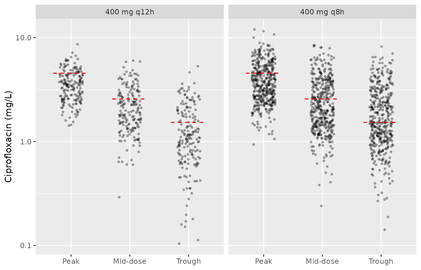
Simulated peak, mid-dose and trough concentrations (points) against the Table 1 observed medians (dashed lines).
Typical-value profiles
ev_typ <- tidyr::crossing(
  BICARBONATE = c(18, 25.7, 39),
  time = c(seq(0, 48, by = 0.1), seq(0, 40, by = 8))
) |>
  distinct() |>
  mutate(id = as.integer(factor(BICARBONATE)), CRCL = 40.83)
dose_t <- seq(0, 40, by = 8)
ev_typ <- ev_typ |>
  mutate(evid = 0L, amt = 0, rate = 0) |>
  bind_rows(
    tidyr::crossing(BICARBONATE = c(18, 25.7, 39), time = dose_t) |>
      mutate(
        id = as.integer(factor(BICARBONATE)), CRCL = 40.83,
        evid = 1L, amt = 400, rate = 800
      )
  ) |>
  group_by(id) |>
  mutate(OCC = pmin(floor(time / 8) + 1, 21)) |>
  ungroup() |>
  mutate(cmt = "central") |>
  arrange(id, time, desc(evid))
sim_typ <- rxode2::rxSolve(
  rxode2::zeroRe(mod), ev_typ,
  keep = "BICARBONATE", returnType = "data.frame"
)
#> Warning: some etas defaulted to non-mu referenced, possible parsing error: etaiov_cl_1, etaiov_cl_2, etaiov_cl_3, etaiov_cl_4, etaiov_cl_5, etaiov_cl_6, etaiov_cl_7, etaiov_cl_8, etaiov_cl_9, etaiov_cl_10, etaiov_cl_11, etaiov_cl_12, etaiov_cl_13, etaiov_cl_14, etaiov_cl_15, etaiov_cl_16, etaiov_cl_17, etaiov_cl_18, etaiov_cl_19, etaiov_cl_20, etaiov_cl_21
#> as a work-around try putting the mu-referenced expression on a simple line
#> ℹ omega/sigma items treated as zero: 'etalcl', 'etalvc', 'etalq', 'etaiov_cl_1', 'etaiov_cl_2', 'etaiov_cl_3', 'etaiov_cl_4', 'etaiov_cl_5', 'etaiov_cl_6', 'etaiov_cl_7', 'etaiov_cl_8', 'etaiov_cl_9', 'etaiov_cl_10', 'etaiov_cl_11', 'etaiov_cl_12', 'etaiov_cl_13', 'etaiov_cl_14', 'etaiov_cl_15', 'etaiov_cl_16', 'etaiov_cl_17', 'etaiov_cl_18', 'etaiov_cl_19', 'etaiov_cl_20', 'etaiov_cl_21'
#> Warning: multi-subject simulation without without 'omega'
ggplot(sim_typ, aes(time, Cc, colour = factor(BICARBONATE))) +
  geom_line() +
  labs(x = "Time (h)", y = "Ciprofloxacin (mg/L)", colour = "Bicarbonate\n(mmol/L)")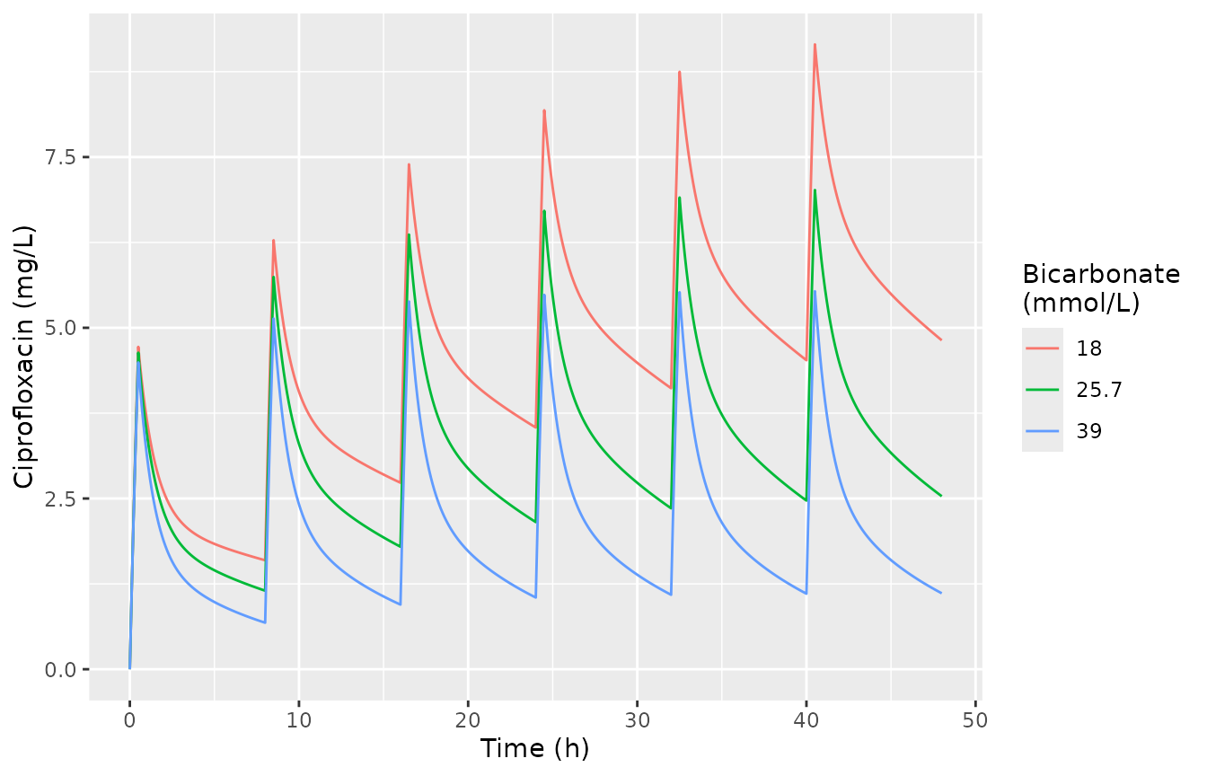
Typical-value concentrations over the first 48 h of 400 mg every 8 h at the lowest, reference and highest plasma bicarbonate (eGFR 40.83 mL/min).
PKNCA: AUC0-24 and probability of target attainment
Section 2.6 simulated 1000 patients per scenario at the lowest and highest observed values of each covariate and counted the fraction achieving AUC0-24/MIC >= 125 mg h/L. The scenarios below use 200 patients each; the covariate not being varied is held at its centring value. Each patient receives 400 mg every 8 h, and PKNCA computes the AUC over the first 24 h. Because the model is linear in dose, the 600 mg and 800 mg AUCs of Figure 4 are the 400 mg AUCs of the same patients scaled by 1.5 and 2.
n_per <- 200
scen <- tibble::tribble(
  ~scenario, ~BICARBONATE, ~CRCL,
  "Bicarbonate 18 mmol/L", 18, 40.83,
  "Bicarbonate 39 mmol/L", 39, 40.83,
  "eGFR 10 mL/min", 25.7, 10,
  "eGFR 150 mL/min", 25.7, 150,
  "Bicarbonate 18 + eGFR 10", 18, 10,
  "Bicarbonate 39 + eGFR 150", 39, 150
) |>
  mutate(sid = row_number())
subj <- tidyr::crossing(scen, rep = seq_len(n_per)) |>
  mutate(id = (sid - 1) * n_per + rep)
ev_pta <- bind_rows(
  tidyr::crossing(subj, k = 1:3) |>
    mutate(time = (k - 1) * 8, OCC = k, amt = 400, rate = 800, evid = 1L),
  tidyr::crossing(subj, time = seq(0, 24, by = 0.25)) |>
    mutate(OCC = pmin(floor(time / 8) + 1, 3), amt = 0, rate = 0, evid = 0L)
) |>
  select(id, scenario, time, BICARBONATE, CRCL, OCC, amt, rate, evid) |>
  mutate(cmt = "central") |>
  arrange(id, time, desc(evid))
rxode2::rxSetSeed(125)
sim_pta <- rxode2::rxSolve(mod, ev_pta, keep = "scenario", returnType = "data.frame")

conc_pta <- sim_pta |>
  filter(!is.na(Cc)) |>
  select(id, scenario, time, Cc)
dose_pta <- ev_pta |>
  filter(evid == 1) |>
  select(id, scenario, time, amt)
nca_pta <- PKNCA::pk.nca(PKNCA::PKNCAdata(
  PKNCA::PKNCAconc(conc_pta, Cc ~ time | scenario + id),
  PKNCA::PKNCAdose(dose_pta, amt ~ time | scenario + id),
  intervals = data.frame(start = 0, end = 24, auclast = TRUE)
))
auc24 <- as.data.frame(nca_pta$result) |>
  filter(PPTESTCD == "auclast") |>
  select(scenario, id, auc = PPORRES)
stopifnot(nrow(auc24) == nrow(scen) * n_per, !anyNA(auc24$auc))
The paper’s PTAs are compared with two readings of “AUC0-24”. The
first is the AUC over the first 24 h of therapy, from the PKNCA results
above. The second is the steady-state daily AUC,
daily dose / CL, whose PTA follows in closed form from the
log-normal clearance (IIV plus IOV) at the typical-value clearance of
each scenario.
om <- ui$omega
sd_cl <- sqrt(om["etalcl", "etalcl"] + om["etaiov_cl_1", "etaiov_cl_1"])
pta_ss <- function(dose_daily, bic, gfr, mic) {
  100 * pnorm((log(dose_daily / (125 * mic)) - log(cl_typ(bic, gfr))) / sd_cl)
}
paper <- tibble::tribble(
  ~scenario, ~dose, ~paper,
  "Bicarbonate 18 mmol/L", 400, 92.8,
  "Bicarbonate 39 mmol/L", 400, 7.3,
  "eGFR 10 mL/min", 400, 71.7,
  "eGFR 150 mL/min", 400, 21.4,
  "Bicarbonate 39 mmol/L", 600, 66.7,
  "Bicarbonate 39 mmol/L", 800, 95.4
)
pta_cmp <- paper |>
  inner_join(scen, by = "scenario") |>
  rowwise() |>
  mutate(
    day1 = 100 * mean(auc24$auc[auc24$scenario == scenario] * dose / 400 / 0.5 >= 125),
    ss = pta_ss(3 * dose, BICARBONATE, CRCL, 0.5)
  ) |>
  ungroup()
stopifnot(nrow(pta_cmp) == nrow(paper))
pta_cmp |>
  transmute(
    scenario, regimen = paste(dose, "mg q8h"), paper, day1, ss
  ) |>
  dplyr::rename(
    "Scenario" = scenario, "Regimen" = regimen,
    "Paper PTA (%)" = paper, "Simulated PTA, first 24 h (%)" = day1,
    "Steady-state PTA, closed form (%)" = ss
  ) |>
knitr::kable(digits = 1)| Scenario | Regimen | Paper PTA (%) | Simulated PTA, first 24 h (%) | Steady-state PTA, closed form (%) |
|---|---|---|---|---|
| Bicarbonate 18 mmol/L | 400 mg q8h | 92.8 | 91.5 | 99.9 |
| Bicarbonate 39 mmol/L | 400 mg q8h | 7.3 | 5.0 | 29.2 |
| eGFR 10 mL/min | 400 mg q8h | 71.7 | 61.0 | 95.6 |
| eGFR 150 mL/min | 400 mg q8h | 21.4 | 13.0 | 56.6 |
| Bicarbonate 39 mmol/L | 600 mg q8h | 66.7 | 55.0 | 78.2 |
| Bicarbonate 39 mmol/L | 800 mg q8h | 95.4 | 95.0 | 95.7 |
At the EUCAST breakpoint of 0.5 mg/L the first-24-h reading reproduces the direction and size of every published covariate and dose effect. It runs uniformly below the paper, by between under 1 and about 12 percentage points depending on the scenario. The steady-state reading does not reproduce the paper: at bicarbonate 39 mmol/L it gives a PTA several-fold higher than the published 7.3%. The paper’s AUC0-24 is therefore the first-day AUC. The remaining uniform shortfall is unexplained; it corresponds to a simulated AUC roughly 5-10% below the paper’s. The parameters were not adjusted to close it.
# Centre and envelope of the first-24-h comparison. The per-scenario Monte
# Carlo SE at n = 200 is up to 3.5 points, so the envelope has headroom.
stopifnot(
  mean(abs(pta_cmp$day1 - pta_cmp$paper)) < 12,
  all(abs(pta_cmp$day1 - pta_cmp$paper) < 20)
)
# Deterministic: the steady-state reading misses the bicarbonate 39 mmol/L
# result by a wide margin, which is what identifies the first-day AUC.
ss_bic39 <- pta_ss(1200, 39, 40.83, 0.5)
stopifnot(ss_bic39 - 7.3 > 15)
Replicate Figures 3 and 4
mics <- c(0.06, 0.125, 0.25, 0.5, 1, 2)
pta_curve <- tidyr::crossing(auc24, mic = mics) |>
  group_by(scenario, mic) |>
  summarise(pta = 100 * mean(auc / mic >= 125), .groups = "drop")
ggplot(pta_curve, aes(mic, pta, colour = scenario)) +
  geom_line() +
  geom_point() +
  geom_hline(yintercept = 90, linetype = "dashed") +
  geom_vline(xintercept = 0.5, linetype = "dotted") +
  scale_x_log10(breaks = mics) +
  labs(x = "MIC (mg/L)", y = "PTA (%)", colour = NULL) +
  theme(legend.position = "bottom") +
  guides(colour = guide_legend(ncol = 2))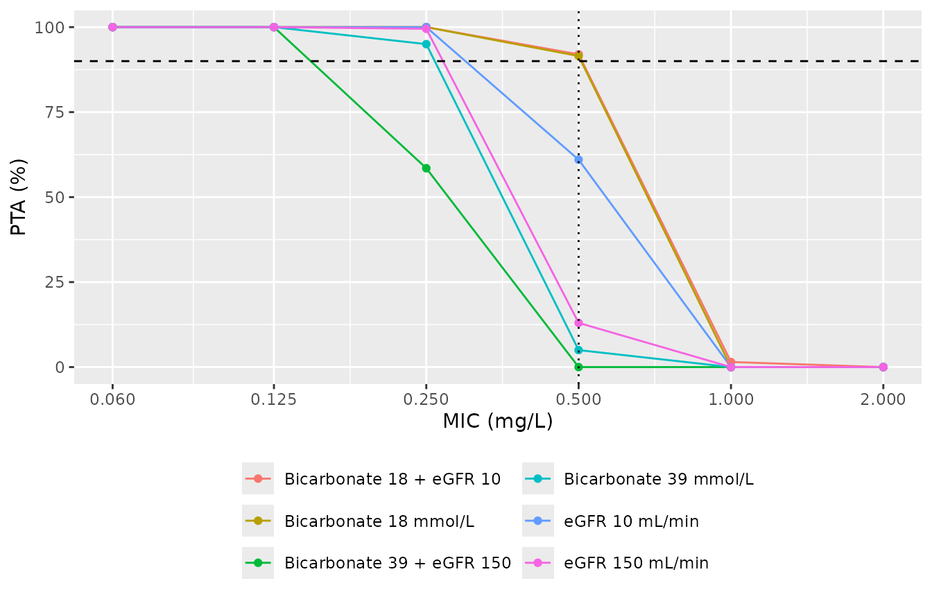
Replicates Figure 3 of Alihodzic 2022: PTA for AUC0-24/MIC >= 125 mg h/L with 400 mg every 8 h across MICs, by covariate scenario. Dotted line: EUCAST breakpoint 0.5 mg/L.
The paper states that at an MIC of 1 mg/L or above the PTA is below 1% for every covariate value in the single-covariate scenarios of Figure 3A-B. It also states that for the combination of high bicarbonate and high eGFR the PTA falls below 75% at 0.25 mg/L and below 1% at 0.5 mg/L.
pta_at <- function(scn, mic_val) {
  v <- pta_curve$pta[pta_curve$scenario == scn & pta_curve$mic == mic_val]
  if (length(v) != 1L) stop("no unique PTA for ", scn, " at MIC ", mic_val)
  v
}
pta_curve |>
  filter(mic %in% c(0.25, 0.5, 1)) |>
  tidyr::pivot_wider(names_from = mic, values_from = pta, names_prefix = "MIC ") |>
  dplyr::rename("Scenario" = scenario) |>
knitr::kable(digits = 1)| Scenario | MIC 0.25 | MIC 0.5 | MIC 1 |
|---|---|---|---|
| Bicarbonate 18 + eGFR 10 | 100.0 | 92.0 | 1.5 |
| Bicarbonate 18 mmol/L | 100.0 | 91.5 | 0.0 |
| Bicarbonate 39 + eGFR 150 | 58.5 | 0.0 | 0.0 |
| Bicarbonate 39 mmol/L | 95.0 | 5.0 | 0.0 |
| eGFR 10 mL/min | 100.0 | 61.0 | 0.0 |
| eGFR 150 mL/min | 99.5 | 13.0 | 0.0 |
stopifnot(
  pta_at("Bicarbonate 39 + eGFR 150", 0.25) < 75,
  pta_at("Bicarbonate 39 + eGFR 150", 0.5) < 5,
  max(pta_curve$pta[pta_curve$mic == 1 & !grepl("\\+", pta_curve$scenario)]) < 10
)
pta_dose <- tidyr::crossing(
  auc24 |> filter(!grepl("\\+", scenario)),
  dose = c(400, 600, 800), mic = mics
) |>
  group_by(scenario, dose, mic) |>
  summarise(pta = 100 * mean(auc * dose / 400 / mic >= 125), .groups = "drop")
ggplot(pta_dose, aes(mic, pta, colour = factor(dose))) +
  geom_line() +
  geom_point() +
  geom_hline(yintercept = 90, linetype = "dashed") +
  geom_vline(xintercept = 0.5, linetype = "dotted") +
  scale_x_log10(breaks = mics) +
  facet_wrap(~scenario) +
  labs(x = "MIC (mg/L)", y = "PTA (%)", colour = "Dose q8h (mg)")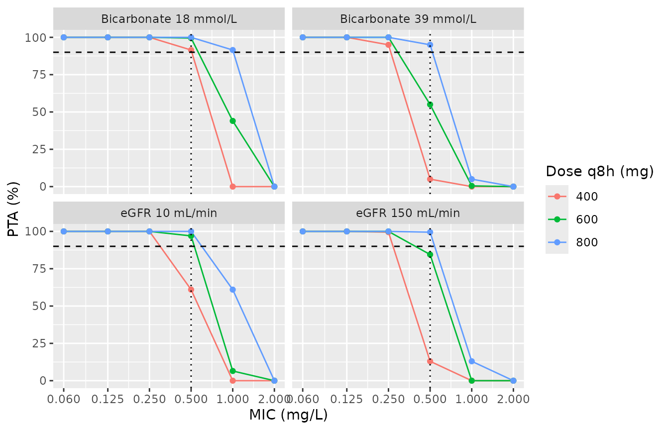
Replicates Figure 4 of Alihodzic 2022: PTA for 400, 600 and 800 mg every 8 h at the lowest and highest covariate values.
Assumptions and deviations
-
Occasion count. The paper defines every
administration as a new occasion but does not state how many occasions
the analysis data held. The model encodes 21, which covers the 7-day
sampling window at 8-hourly dosing; all 21 share the single estimated
IOV variance. Records with
OCCoutside 1-21 carry no IOV. -
eGFR units. The retained eGFR is CKD-EPI computed
with the patient’s actual body surface area, so it is in absolute mL/min
rather than the usual mL/min/1.73 m^2. It is carried in the
CRCLcolumn. Users must de-index a reported eGFR (multiply by BSA / 1.73) before supplying it. - Covariate centring. Equation 1 centres on 25.7 mmol/L and 40.83 mL/min, which differ from the Table 1 per-patient medians (26.6 mmol/L, 46.8 mL/min). The equation’s values are used. They are probably medians over records rather than over patients, but the paper does not say.
- Range of the bicarbonate effect. The linear bicarbonate term describes the alkalotic side of the observed 18-39 mmol/L range only. The Discussion notes that the effect of acidosis was not characterised. Clearance reaches zero at 8.2 mmol/L, so the model should not be extrapolated far below the observed range.
-
Residual error. Table 2 reports the proportional
error as 12.1% CV and states that CVs were obtained as
sqrt(exp(OMEGA) - 1). The model usespropSd = 0.121; back-transforming through that formula would give 0.1206, which is immaterial. - PTA reading. The paper does not state the AUC0-24 window. The first-24-h window reproduces its PTAs, while the steady-state window does not (see the table above). The paper’s other covariate was presumably held at a fixed value in the single-covariate scenarios. The value is not reported, and the centring value is used here. Holding it at the Table 1 median instead lowers the PTAs a further 1-6 points.
- Virtual cohort. Bicarbonate and eGFR are drawn independently as log-normals matched to the Table 1 medians and IQRs. The paper does not report their correlation or the per-patient sampling days.