Abrocitinib platelet time-course (Wojciechowski 2022) • nlmixr2lib

Model and source

Citation: Wojciechowski J, Malhotra BK, Wang X, Fostvedt L, Valdez H, Nicholas T. Population pharmacokinetic-pharmacodynamic modelling of platelet time-courses following administration of abrocitinib. Br J Clin Pharmacol. 2022;88(8):3856-3871. doi:10.1111/bcp.15334. PK structure from Wojciechowski J et al. Population Pharmacokinetics of Abrocitinib in Healthy Individuals and Patients with Psoriasis or Atopic Dermatitis. Clin Pharmacokinet. 2022;61:709-723. doi:10.1007/s40262-021-01104-z; see modellib(‘Wojciechowski_2022_abrocitinib’).
Description: Population PK-PD model of the platelet time-course after oral abrocitinib (JAK1 inhibitor) in adolescents and adults with atopic dermatitis or psoriasis (Wojciechowski 2022, Br J Clin Pharmacol). A Friberg semi-mechanistic myelosuppression model (proliferating pool, three transit compartments and circulating platelets, mean transit time 7.21 days, feedback exponent 0.232) in which abrocitinib concentration inhibits platelet proliferation by an Emax function. Emax scales with the individual baseline platelet count (power -1.11) and wanes with time on treatment (tachyphylaxis half-life 151 days). Baseline platelet count depends on baseline white blood cell count, haematocrit, age, sex and psoriasis. The abrocitinib concentrations come from the companion Wojciechowski 2022 population PK model, carried here unchanged.
Article: https://doi.org/10.1111/bcp.15334 (open access, Br J Clin Pharmacol 2022;88(8):3856-3871). No correction notice was listed in Europe PMC as of 2026-10-09.

The paper fits a Friberg semi-mechanistic myelosuppression model to platelet counts. The abrocitinib concentration that drives it comes from the population PK model of the same group, which is packaged separately as modellib("Wojciechowski_2022_abrocitinib") and has its own vignette. This file carries that PK model unchanged and adds the platelet layer, so a single rxSolve() gives both abrocitinib concentration (Cc, ng/mL) and platelet count (PLT, x 1000/uL, which equals 10^9/L).

Population

The platelet model was fitted to 12 189 platelet counts from 2333 patients in five studies: the phase II psoriasis study B7451005 (n = 59), the phase IIb atopic dermatitis (AD) study B7451006 (n = 269) and the phase III AD studies JADE MONO-1, JADE MONO-2 and JADE REGIMEN (n = 387, 391 and 1236; Table A1). Of the 2333 patients, 2274 had AD (340 of them adolescents aged 12-17 years) and 59 had psoriasis. Median age was 30 years (range 12-84), median weight 73 kg (34-204) and 44.4% were female; 71.8% were White, 17.8% Asian, 7.6% Black, 2.3% other race and 0.6% unknown. Median baseline platelet count was 274 x 1000/uL (118-651), white blood cell count 7 x 1000/uL and haematocrit 43% (Table 1). Patients received placebo (n = 224) or abrocitinib 10, 30, 100, 200 or 400 mg once daily or 200 mg twice daily for 4-12 weeks, with platelet counts up to week 16.

str(readModelDb("Wojciechowski_2022_abrocitinib_platelets")()$population)
#> List of 15
#>  $ species           : chr "human"
#>  $ n_subjects        : int 2333
#>  $ n_studies         : int 5
#>  $ n_observations    : int 12189
#>  $ age_range         : chr "12-84 years"
#>  $ age_median        : chr "30 years"
#>  $ weight_range      : chr "34-204 kg"
#>  $ weight_median     : chr "73 kg"
#>  $ sex_female_pct    : num 44.4
#>  $ race_ethnicity    : Named num [1:5] 71.8 17.8 7.6 2.3 0.6
#>   ..- attr(*, "names")= chr [1:5] "White" "Asian" "Black" "Other" ...
#>  $ disease_state     : chr "Moderate-to-severe atopic dermatitis (n = 2274, including 340 adolescents aged 12-17 years) and moderate-to-sev"| __truncated__
#>  $ dose_range        : chr "Placebo (n = 224) or oral abrocitinib 10, 30, 100, 200 or 400 mg once daily or 200 mg twice daily for 4-12 weeks"
#>  $ regions           : chr "Multinational (includes 44 Japanese patients)"
#>  $ baseline_platelets: chr "Median 274 x 1000/uL (range 118-651)"
#>  $ notes             : chr "Two phase II studies (B7451005 psoriasis, B7451006 atopic dermatitis) and three phase III atopic dermatitis stu"| __truncated__

Source trace

Platelet-model values are from Table 2 of the Br J Clin Pharmacol paper and equations from its Methods. The abrocitinib PK block is documented in the companion vignette and in the comments of the model file (marked CPK).

Equation / parameter	Value	Source location
`lrbase` (CIRC0)	log(270) x 1000/uL	Table 2 ‘Baseline platelet count’
`lgamma`	log(0.232)	Table 2 ‘Feedback exponent (GAM)’
`lmtt`	log(7.21 x 24) h	Table 2 ‘Mean transit time (MTT; days)’ = 7.21
`lemax`	log(0.109)	Table 2 ‘Maximum drug effect on platelet proliferation’
`lec50`	log(55.3) ng/mL	Table 2 ‘Concentration at 50% of maximum drug effect’
`e_rbase_emax`	-1.11	Table 2 ‘Effect of CIRC0 on Emax’; Results 3.2 (power model referenced to the typical CIRC0)
`emax_exp_famp`	-1, fixed	Results 3.2: DELTATCPX estimated at 0.991, then fixed to 1
`lemax_exp_kdes`	log(ln 2 / (151 x 24)) 1/h	Table 2 ‘Half-life of tachyphylaxis (kTCPX; days)’ = 151
`e_wbc_rbase`	0.199, reference 6.9 x 1000/uL	Table 2
`e_sexf_rbase`	0.0584	Table 2 ‘Effect of female sex on CIRC0’
`e_age_rbase`	-0.0695, reference 30 years	Table 2
`e_hct_rbase`	-0.203, reference 43%	Table 2
`e_dis_psoriasis_rbase`	-0.118	Table 2 ‘Effect of psoriasis patients on CIRC0’
`etalrbase`	0.175^2	Table 2 ‘omega CIRC0 (% CV)’ = 17.5; footnote CV = sqrt(omega^2) x 100
`propSd_PLT`, `addSd_PLT`	0.120, 16.4 x 1000/uL	Table 2 RUV PRO / RUV ADD (SDs; EPS variance fixed to 1)
`d/dt(prol)` … `d/dt(circ)`	n/a	Equations 1-5
`ktr = 4 / mtt`	n/a	Equation 6 with n = 3; kPROL = kTR = kCIRC (Methods 2.3)
`emax` time course	`emax * (1 + emax_exp_famp * (1 - exp(-emax_exp_kdes * t)))`	Equation 7 with Emax(t) = Emax x (1 - TCPX)
covariates on CIRC0	power (continuous), 1 + theta (categorical)	Equations 9 and 10
`PLT ~ add(addSd_PLT) + prop(propSd_PLT)`	n/a	Table 2 footnote, `RUVSD = sqrt(RUVPRO^2 * IPRE^2 + RUVADD^2)`
PK (`Cc` and its parameters)	n/a	`modellib("Wojciechowski_2022_abrocitinib")`; Methods 2.3

Dosing the model

Dosing follows the PK model: every administration is two records with the same amount, one into depot with rate = 0 and one into central with rate = -1. DOSE_ABROCITINIB_MG is the amount per administration, DOSE_ABROCITINIB_MGD the daily dose, and MULTI_DOSE switches from 0 to 1 at the second dose. The time-dependent PK clearance and the tachyphylaxis term both run on the solver time, so the first dose must be at t = 0.

Because the model has two endpoints (Cc and PLT), observation rows carry dvid. Here they are written on the circ state with dvid = 2 (the platelet endpoint); the algebraic Cc is returned on the same rows.

The paper’s reference patient is a White, 30-year-old male with AD weighing 70 kg; the platelet covariates are set to the Table 2 reference values (white blood cell count 6.9 x 1000/uL, haematocrit 43%), so that patient’s typical baseline is 270 x 1000/uL. The phase III tablet is used throughout.

reference_covariates <- function(...) {
  base <- list(
    WT = 70, SEXF = 0, RACE_ASIAN = 0, RACE_OTHER = 0, ADOLESCENT = 0,
    DIS_PSORIASIS = 0, DIS_ATOPIC_DERMATITIS = 1,
    HEPIMP_MILD = 0, HEPIMP_MOD = 0,
    CONMED_RIFAMPICIN = 0, CONMED_FLUCONAZOLE = 0, CONMED_FLUVOXAMINE = 0,
    FED_HIGHFAT = 0,
    FORM_ABROCITINIB_SUSP = 0, FORM_ABROCITINIB_TAB_PH2B = 0,
    FORM_ABROCITINIB_TAB_PH3 = 1,
    STUDY_B7451005 = 0, STUDY_B7451006 = 0, STUDY_B7451012 = 0,
    STUDY_B7451043 = 0,
    AGE = 30, WBC = 6.9, HCT = 43,
    DOSE_ABROCITINIB_MG = 200, DOSE_ABROCITINIB_MGD = 200
  )
  as.data.frame(utils::modifyList(base, list(...)))
}

# One subject: once-daily doses on the days in `dose_days` (day 0 = first
# dose), each as a depot record and a rate = -1 central record, plus platelet
# observations at `obs_times` (h).
regimen_events <- function(id, cov, dose_days, obs_times) {
  dose_times <- dose_days * 24
  amt <- cov$DOSE_ABROCITINIB_MG
  doses <- dplyr::bind_rows(
    data.frame(time = dose_times, amt = amt, evid = 1L, cmt = "depot", rate = 0),
    data.frame(time = dose_times, amt = amt, evid = 1L, cmt = "central", rate = -1)
  )
  obs <- data.frame(
    time = obs_times, amt = 0, evid = 0L, cmt = "circ", rate = 0, dvid = 2L
  )
  ev <- dplyr::bind_rows(doses, obs) |>
    dplyr::arrange(time, dplyr::desc(evid)) |>
    dplyr::mutate(id = id)
  ev <- cbind(ev, cov[rep(1, nrow(ev)), , drop = FALSE])
  ev$MULTI_DOSE <- as.integer(ev$time > min(dose_times))
  ev
}

mod <- readModelDb("Wojciechowski_2022_abrocitinib_platelets")
mod_typical <- rxode2::zeroRe(mod)
#> ℹ parameter labels from comments will be replaced by 'label()'

Typical patient: abrocitinib exposure

Results 3.2 states that for the average AD patient on 200 mg once daily the steady-state concentration ranges from 13.0 to 1181 ng/mL and stays above the EC50 of 55.3 ng/mL for 15.3 hours of each 24-hour interval. The PK layer is checked against those numbers with PKNCA over day 84.

day84 <- seq(83 * 24, 84 * 24, by = 0.05)
ev_pk <- dplyr::bind_rows(
  regimen_events(1, reference_covariates(DOSE_ABROCITINIB_MG = 100, DOSE_ABROCITINIB_MGD = 100),
    dose_days = 0:83, obs_times = c(0, day84)
  ) |> dplyr::mutate(treatment = "100 mg QD"),
  regimen_events(2, reference_covariates(),
    dose_days = 0:83, obs_times = c(0, day84)
  ) |> dplyr::mutate(treatment = "200 mg QD")
)
sim_pk <- rxode2::rxSolve(
  mod_typical, ev_pk, keep = "treatment", returnType = "data.frame"
)
#> ℹ omega/sigma items treated as zero: 'etalcl', 'etalvc', 'etalrbase'
#> Warning: multi-subject simulation without without 'omega'

conc_pk <- sim_pk |>
  dplyr::filter(!is.na(Cc)) |>
  dplyr::select(id, treatment, time, Cc)
dose_pk <- ev_pk |>
  dplyr::filter(evid == 1, cmt == "depot") |>
  dplyr::select(id, treatment, time, amt)
nca_pk <- PKNCA::pk.nca(PKNCA::PKNCAdata(
  PKNCA::PKNCAconc(conc_pk, Cc ~ time | treatment + id),
  PKNCA::PKNCAdose(dose_pk, amt ~ time | treatment + id),
  intervals = data.frame(
    start = 83 * 24, end = 84 * 24, cmax = TRUE, cmin = TRUE, auclast = TRUE
  )
))
nca_pk_tbl <- as.data.frame(nca_pk) |>
  dplyr::filter(PPTESTCD %in% c("cmax", "cmin", "auclast"))

time_above_ec50 <- conc_pk |>
  dplyr::filter(time >= 83 * 24) |>
  dplyr::group_by(treatment) |>
  dplyr::summarise(hours = sum(Cc[-1] > 55.3) * 0.05, .groups = "drop")

cmp_pk <- nlmixr2lib::ncaComparisonTable(
  simulated = nca_pk_tbl |> dplyr::filter(treatment == "200 mg QD"),
  reference = data.frame(treatment = "200 mg QD", cmax = 1181, cmin = 13.0),
  by = "treatment",
  units = c(cmax = "ng/mL", cmin = "ng/mL")
)
knitr::kable(cmp_pk, caption = "Typical AD patient, 200 mg once daily, day 84 (Results 3.2).")

Typical AD patient, 200 mg once daily, day 84 (Results 3.2).
NCA parameter	treatment	Reference	Simulated	% diff
Cmax (ng/mL)	200 mg QD	1180	1180	-0.4%
Cmin (ng/mL)	200 mg QD	13	12.6	-3.4%

knitr::kable(
  time_above_ec50 |>
    dplyr::mutate(hours = round(hours, 1)) |>
    dplyr::rename("Regimen" = treatment, "Hours above EC50 per day" = hours),
  caption = "Time above EC50 at steady state; the paper reports 15.3 h for 200 mg."
)

Time above EC50 at steady state; the paper reports 15.3 h for 200 mg.
Regimen	Hours above EC50 per day
100 mg QD	10.2
200 mg QD	15.2

sim_200 <- nca_pk_tbl |>
  dplyr::filter(treatment == "200 mg QD") |>
  dplyr::select(PPTESTCD, PPORRES) |>
  tidyr::pivot_wider(names_from = PPTESTCD, values_from = PPORRES)
stopifnot(
  abs(sim_200$cmax / 1181 - 1) < 0.05,
  abs(sim_200$cmin / 13.0 - 1) < 0.10,
  abs(time_above_ec50$hours[time_above_ec50$treatment == "200 mg QD"] - 15.3) < 1
)

Typical patient: platelet time-course and missed doses

The paper reports the platelet nadir 24 days after starting 200 mg once daily (Results 3.3), and Figure 4 shows the population-typical 16-week course (12 weeks of 200 mg once daily, then 4 weeks off) with seven consecutive doses missed in week 2, 3, 4 or 8. The same scenarios are simulated below with the typical-value model.

obs_days <- seq(0, 112, by = 0.25)
missed <- list(
  "No missed doses" = integer(0),
  "Missed week 2 doses" = 7:13,
  "Missed week 3 doses" = 14:20,
  "Missed week 4 doses" = 21:27,
  "Missed week 8 doses" = 49:55
)
ev_f4 <- dplyr::bind_rows(lapply(seq_along(missed), function(i) {
  regimen_events(i, reference_covariates(),
    dose_days = setdiff(0:83, missed[[i]]), obs_times = obs_days * 24
  ) |>
    dplyr::mutate(scenario = names(missed)[i])
}))
sim_f4 <- rxode2::rxSolve(
  mod_typical, ev_f4, keep = "scenario", returnType = "data.frame"
) |>
  dplyr::mutate(day = time / 24)
#> ℹ omega/sigma items treated as zero: 'etalcl', 'etalvc', 'etalrbase'
#> Warning: multi-subject simulation without without 'omega'

no_miss <- sim_f4 |> dplyr::filter(scenario == "No missed doses")
f4_plot <- dplyr::bind_rows(lapply(names(missed)[-1], function(s) {
  dplyr::bind_rows(
    sim_f4 |> dplyr::filter(scenario == s) |> dplyr::mutate(line = "Missed dosing"),
    no_miss |> dplyr::mutate(line = "No missed dosing")
  ) |>
    dplyr::mutate(panel = s)
}))
ggplot(f4_plot, aes(day, PLT, colour = line)) +
  annotate("rect", xmin = 84, xmax = 112, ymin = -Inf, ymax = Inf, alpha = 0.2, fill = "green4") +
  geom_line() +
  facet_wrap(~panel) +
  scale_colour_manual(values = c("Missed dosing" = "black", "No missed dosing" = "red")) +
  scale_x_continuous(breaks = seq(0, 112, by = 14)) +
  labs(
    x = "Time after first dose (days)", y = "Platelet count (x 1000/uL)", colour = NULL,
    caption = "Replicates Figure 4 of Wojciechowski 2022 (shaded: washout)."
  ) +
  theme_bw() +
  theme(legend.position = "bottom")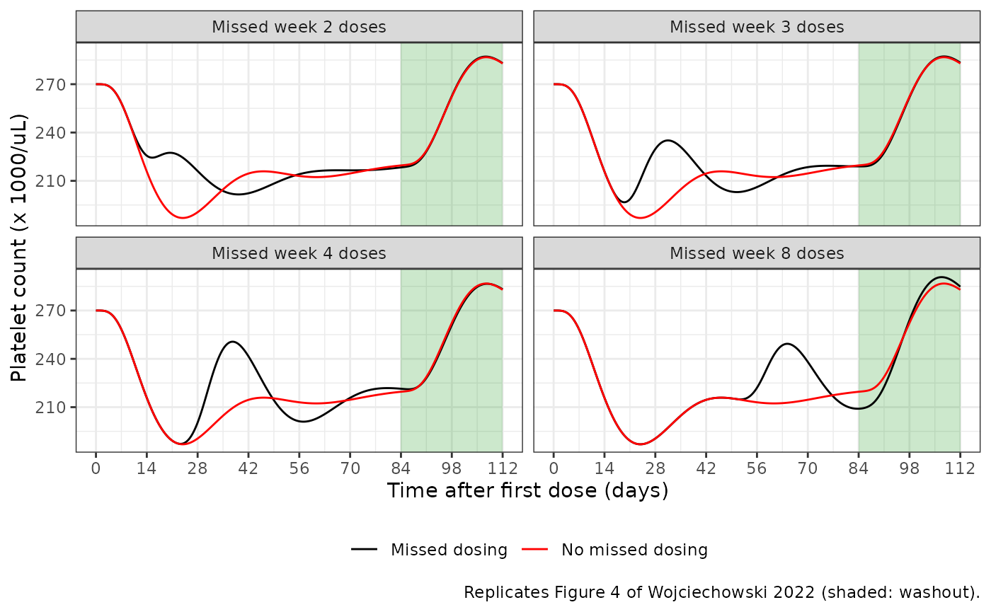


typ_summary <- no_miss |>
  dplyr::summarise(
    nadir_day = day[which.min(PLT)],
    nadir = min(PLT),
    week12 = PLT[day == 84],
    peak_washout = max(PLT[day > 84])
  )
knitr::kable(
  typ_summary |>
    dplyr::mutate(dplyr::across(dplyr::everything(), \(x) round(x, 1))) |>
    dplyr::rename(
      "Nadir day" = nadir_day, "Nadir (x 1000/uL)" = nadir,
      "Week 12 (x 1000/uL)" = week12, "Washout peak (x 1000/uL)" = peak_washout
    ),
  caption = "Typical AD patient on 200 mg once daily, from a baseline of 270 x 1000/uL."
)

Typical AD patient on 200 mg once daily, from a baseline of 270 x 1000/uL.
Nadir day	Nadir (x 1000/uL)	Week 12 (x 1000/uL)	Washout peak (x 1000/uL)
24	187	219.6	286.7


missed3 <- sim_f4 |> dplyr::filter(scenario == "Missed week 3 doses", day < 40)
nadir_day_missed3 <- missed3$day[which.min(missed3$PLT)]

The typical nadir falls on day 24 (paper: day 24). When week 3 is missed the first nadir moves earlier, to day 19.5 (paper: day 20).

stopifnot(
  abs(typ_summary$nadir_day - 24) <= 1,
  abs(nadir_day_missed3 - 20) <= 1.5
)

Tachyphylaxis

The Discussion states that the drug effect on platelet proliferation falls by 32% after 12 weeks and is essentially gone after about 108 weeks (about five half-lives). With emax_exp_famp = -1 the remaining fraction of Emax is exp(-emax_exp_kdes * t):

kdes <- log(2) / (151 * 24)
lost_12wk <- 1 - exp(-kdes * 84 * 24)
lost_108wk <- 1 - exp(-kdes * 108 * 7 * 24)
c(lost_at_12_weeks = lost_12wk, lost_at_108_weeks = lost_108wk)
#>  lost_at_12_weeks lost_at_108_weeks 
#>         0.3199519         0.9688931
stopifnot(abs(lost_12wk - 0.32) < 0.01, lost_108wk > 0.95)

Covariate effects on baseline platelet count

The Discussion gives three readings of the covariate model: females have a 6% higher baseline than males, and 14-year-old (5th percentile) and 64-year-old (95th percentile) patients have about 5% higher and lower baselines than a 30-year-old.

ini_vals <- rxode2::rxode(mod)$theta
#> ℹ parameter labels from comments will be replaced by 'label()'
cov_check <- c(
  female = 1 + ini_vals[["e_sexf_rbase"]],
  age_14 = (14 / 30)^ini_vals[["e_age_rbase"]],
  age_64 = (64 / 30)^ini_vals[["e_age_rbase"]]
)
round(cov_check, 3)
#> female age_14 age_64 
#>  1.058  1.054  0.949
stopifnot(
  abs(cov_check[["female"]] - 1.06) < 0.005,
  abs(cov_check[["age_14"]] - 1.05) < 0.01,
  abs(cov_check[["age_64"]] - 0.95) < 0.01
)

Probability of thrombocytopaenia (Table 3, Figure 2)

The paper simulated 1000 typical patients per scenario (White, 30-year-old, male, AD, 70 kg) at baseline platelet counts of 170, 220 and 270 x 1000/uL, on 100 or 200 mg once daily for 12 weeks, with IIV on the PK and PD parameters and residual error. Here each scenario has 200 patients.

Each patient’s baseline is held at the scenario value: the CIRC0 random effect is fixed to zero and the white blood cell count is set so that the typical CIRC0 equals the target, WBC = 6.9 * (target / 270)^(1 / 0.199). White blood cell count is used because it is the one continuous covariate on CIRC0. The reference of the Emax power term stays at the estimated 270. The PK random effects and the residual error are kept. Holding the baseline fixed is the reading under which the 100 mg probabilities below agree with Table 3. Keeping the 17.5% IIV on CIRC0 instead roughly doubles the probability of a nadir below 150 x 1000/uL at a baseline of 270 (about 20% against the paper’s 7%). The nadir is the simulated observation at the time of each patient’s predicted nadir, and changes are from the scenario baseline.

n_per_arm <- 200
scen <- expand.grid(dose = c(100, 200), baseline = c(170, 220, 270))
ev_t3 <- dplyr::bind_rows(lapply(seq_len(nrow(scen)), function(k) {
  cov <- reference_covariates(
    DOSE_ABROCITINIB_MG = scen$dose[k], DOSE_ABROCITINIB_MGD = scen$dose[k],
    WBC = 6.9 * (scen$baseline[k] / 270)^(1 / 0.199)
  )
  # Daily observations from day 1. The baseline is the model's rbase; an
  # observation row at t = 0 coincides with the zero-order dose record of
  # the 200 mg arms and returns no simulated residual there.
  one <- regimen_events(1, cov, dose_days = 0:83, obs_times = seq(1, 84, by = 1) * 24)
  dplyr::bind_rows(lapply(seq_len(n_per_arm), function(i) {
    one |> dplyr::mutate(
      id = (k - 1) * n_per_arm + i,
      dose = paste(scen$dose[k], "mg"),
      baseline = scen$baseline[k]
    )
  }))
}))

mod_fixed_baseline <- rxode2::rxode(mod) |>
  rxode2::ini(etalrbase = fix(0))
#> ℹ parameter labels from comments will be replaced by 'label()'
#> ℹ fix `etalrbase` to `0.030625`
#> ℹ change initial estimate of `etalrbase` to `0`
rxode2::rxSetSeed(20221025)
sim_t3 <- rxode2::rxSolve(
  mod_fixed_baseline, ev_t3, keep = c("dose", "baseline"), returnType = "data.frame"
)
#> ℹ omega/sigma items treated as zero: 'etalrbase'

per_patient <- sim_t3 |>
  dplyr::group_by(id, dose, baseline) |>
  dplyr::summarise(
    base_i = rbase[1],
    nadir = sim[which.min(circ)],
    week12 = sim[time == 84 * 24],
    .groups = "drop"
  )
stopifnot(!anyNA(sim_t3$sim), !anyNA(per_patient$nadir), !anyNA(per_patient$week12))

t3 <- per_patient |>
  dplyr::group_by(dose, baseline) |>
  dplyr::summarise(
    nadir_change = median(nadir - base_i),
    week12_change = median(week12 - base_i),
    p_any_grade_nadir = 100 * mean(nadir < 150),
    p_below_100_nadir = 100 * mean(nadir < 100),
    .groups = "drop"
  )

published <- tibble::tribble(
  ~dose, ~baseline, ~pub_nadir_change, ~pub_week12_change, ~pub_any_grade, ~pub_below_100,
  "100 mg", 170, -63.9, -38.8, 92.1, 40.9,
  "100 mg", 220, -65.4, -38.2, 43.5, 4.0,
  "100 mg", 270, -66.0, -37.0, 7.0, 0.2,
  "200 mg", 170, -70.1, -44.5, 95.5, 50.1,
  "200 mg", 220, -73.4, -46.6, 53.9, 6.3,
  "200 mg", 270, -71.5, -42.6, 8.6, 0.4
)
t3_cmp <- published |>
  dplyr::left_join(t3, by = c("dose", "baseline")) |>
  dplyr::mutate(nadir_pct_diff = 100 * (nadir_change / pub_nadir_change - 1))

knitr::kable(
  t3_cmp |>
    dplyr::transmute(
      "Dose" = dose,
      "Baseline (x 1000/uL)" = baseline,
      "Nadir change, model" = round(nadir_change, 1),
      "Nadir change, paper" = pub_nadir_change,
      "Week 12 change, model" = round(week12_change, 1),
      "Week 12 change, paper" = pub_week12_change,
      "P(<150) at nadir, model (%)" = round(p_any_grade_nadir, 1),
      "P(<150) at nadir, paper (%)" = pub_any_grade,
      "P(<100) at nadir, model (%)" = round(p_below_100_nadir, 1),
      "P(<100) at nadir, paper (%)" = pub_below_100
    ),
  caption = paste(
    "Replicates Table 3 of Wojciechowski 2022. Changes are medians in",
    "x 1000/uL. Paper P(<150) is the sum of the Grade 1-4 rows as given in",
    "Results 3.3 (92.1%, 43.5%, 7.0%; 95.5%, 53.9%, 8.6%)."
  )
)

Replicates Table 3 of Wojciechowski 2022. Changes are medians in x 1000/uL. Paper P(<150) is the sum of the Grade 1-4 rows as given in Results 3.3 (92.1%, 43.5%, 7.0%; 95.5%, 53.9%, 8.6%).
Dose	Baseline (x 1000/uL)	Nadir change, model	Nadir change, paper	Week 12 change, model	Week 12 change, paper	P(<150) at nadir, model (%)	P(<150) at nadir, paper (%)	P(<100) at nadir, model (%)	P(<100) at nadir, paper (%)
100 mg	170	-63.3	-63.9	-35.9	-38.8	94.5	92.1	41.0	40.9
100 mg	220	-66.9	-65.4	-40.5	-38.2	45.0	43.5	4.0	4.0
100 mg	270	-64.9	-66.0	-39.7	-37.0	6.0	7.0	0.0	0.2
200 mg	170	-82.4	-70.1	-52.6	-44.5	98.0	95.5	71.5	50.1
200 mg	220	-78.5	-73.4	-50.8	-46.6	61.0	53.9	7.0	6.3
200 mg	270	-79.5	-71.5	-47.8	-42.6	12.5	8.6	0.0	0.4

sim_t3 |>
  dplyr::mutate(day = time / 24) |>
  dplyr::group_by(dose, baseline, day) |>
  dplyr::summarise(
    median = median(sim), lo = quantile(sim, 0.05), hi = quantile(sim, 0.95),
    .groups = "drop"
  ) |>
  ggplot(aes(day, median)) +
  geom_ribbon(aes(ymin = lo, ymax = hi), fill = "lightblue") +
  geom_line(colour = "blue") +
  geom_hline(yintercept = 150, linetype = "dashed") +
  geom_hline(yintercept = 100, linetype = "dashed", colour = "red") +
  facet_grid(dose ~ paste("Baseline:", baseline)) +
  scale_x_continuous(breaks = seq(0, 84, by = 14)) +
  labs(
    x = "Time after first dose (days)", y = "Platelet count (x 1000/uL)",
    caption = "Replicates Figure 2A-B of Wojciechowski 2022: median and 90% PI of simulated observations."
  ) +
  theme_bw()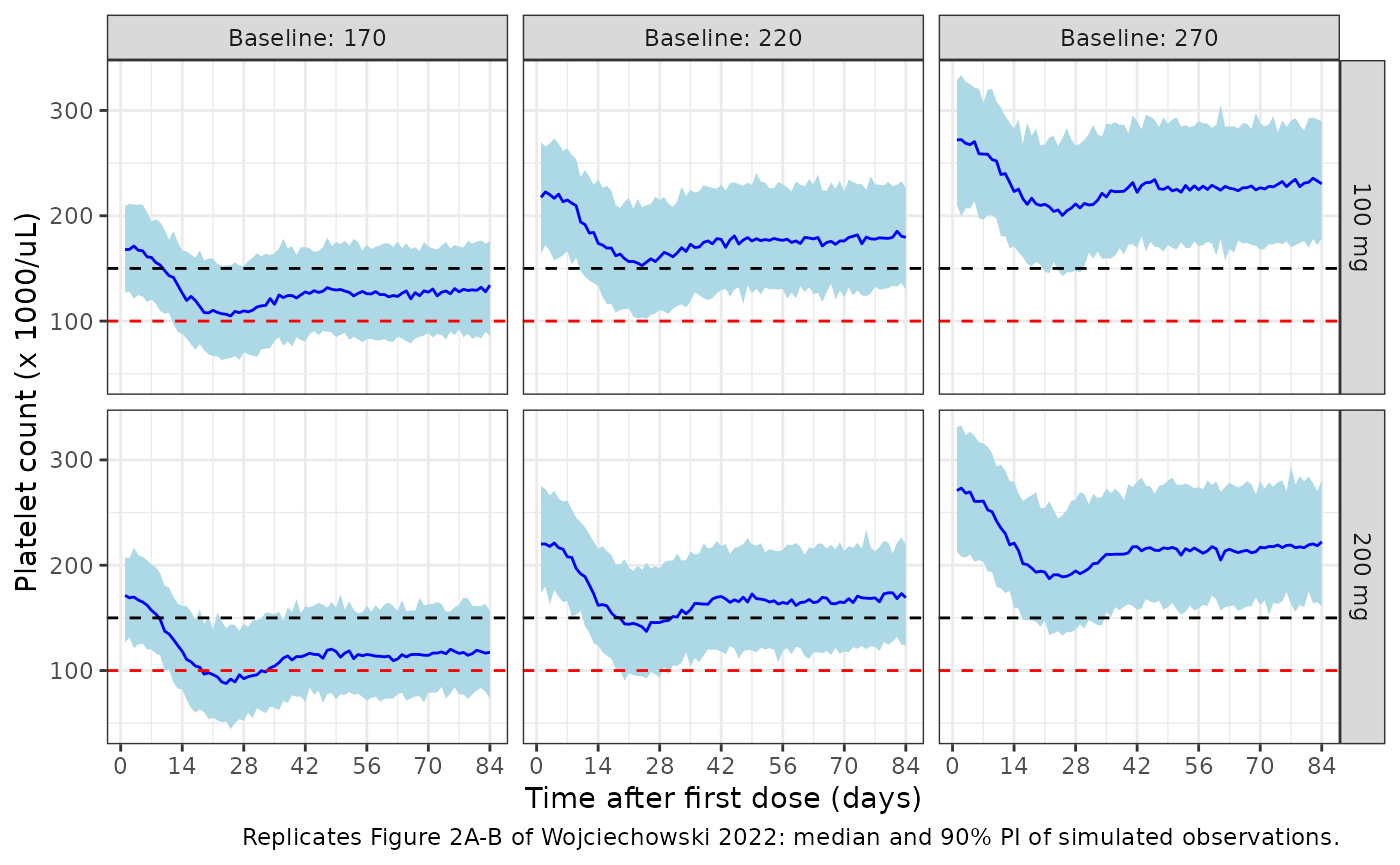

# Medians and proportions of 200 simulated patients per scenario. The 100 mg
# nadir changes sit within ~5% of the paper and the 200 mg ones 7-20% deeper
# (see Assumptions and deviations); a mis-transcribed EC50, Emax or MTT moves
# every row by tens of percent. The binomial SD of a proportion near 50% with
# 200 patients is 3.5 percentage points, so 12 points leaves room for the
# cohort draw while still catching a baseline-IIV or residual-error mistake
# (keeping the CIRC0 IIV moves the 270 baseline row from ~6% to ~20%).
p100 <- t3_cmp[t3_cmp$dose == "100 mg", ]
stopifnot(
  abs(median(p100$nadir_pct_diff)) < 10,
  max(abs(t3_cmp$nadir_pct_diff)) < 30,
  abs(median(t3_cmp$week12_change / t3_cmp$pub_week12_change - 1)) < 0.25,
  max(abs(p100$p_any_grade_nadir - p100$pub_any_grade)) < 12
)

Assumptions and deviations

Tachyphylaxis gate. Equation 7 sets TCPX to 0 when the dose amount is 0 (placebo, or drug withdrawn). Here the term depends only on the time since the first dose. For placebo the concentration is zero, so the term has no effect. During a dosing gap it only acts on the small amount of drug still circulating. After dosing restarts, the paper describes the effect as diminished compared with the first dose, which matches the time-since-first-dose reading used here.
How tachyphylaxis enters Emax. The paper describes TCPX as an exponential function “proportional to Emax” without printing the product. Emax(t) = Emax x (1 - TCPX) is used. It reproduces the Discussion’s statements that the effect falls by 32% after 12 weeks and is gone after about 108 weeks.
Effect of CIRC0 on Emax uses the individual model baseline, including covariates and IIV, divided by the typical estimate of 270 (Results 3.2, “referenced to the population typical estimate for baseline platelet count”).
Baseline covariates. White blood cell count and haematocrit are baseline values. Table 2 gives their reference values (6.9 x 1000/uL and 43%), and Table 1 gives the median age of 30 years.
Psoriasis. The platelet psoriasis effect is relative to AD (every patient in the platelet analysis had one of the two). The PK layer’s shared psoriasis/AD bioavailability shift is relative to healthy volunteers. Simulate AD patients with DIS_ATOPIC_DERMATITIS = 1 and psoriasis patients with DIS_PSORIASIS = 1.
Sequential fit. The paper used empirical Bayes estimates of the PK parameters as fixed inputs. When this model is simulated, the PK random effects are drawn together with the CIRC0 random effect. This matches how the paper itself simulated new patients (Methods 2.8).
Table 3 baselines. The paper’s Methods mention IIV in “PK and PD parameters”, but the PD model’s only random effect is on CIRC0, and the scenarios are described as typical individuals with a given baseline. The replication holds each baseline at the scenario value (CIRC0 random effect fixed to zero, target set through the white blood cell count). With that design the 100 mg probabilities of a nadir below 150 and below 100 x 1000/uL match Table 3 to within a few percentage points.
200 mg nadir depth. The PK layer reproduces the paper’s typical steady-state concentrations at 200 mg (Cmax, trough and time above EC50), and the 100 mg platelet results reproduce Table 3. At 200 mg, however, the simulated nadir is deeper than published: the typical nadir from 270 is about 187 x 1000/uL against about 199 read from Figure 4, and the Table 3 median nadir changes are 7-18% larger, with probabilities of a nadir below 150 x 1000/uL a few points higher. Every parameter was checked against Table 2, and no transcription error was found that would explain it. The model is not tuned to close the gap.