Upifitamab rilsodotin AF-HPA payload drug interactions (Kumar 2025)
Source:vignettes/articles/Kumar_2025_upifitamabRilsodotin.Rmd
Kumar_2025_upifitamabRilsodotin.RmdModel and source
Kumar 2025 built a Simcyp physiologically based pharmacokinetic (PBPK) model for upifitamab rilsodotin, a NaPi2b-targeted antibody-drug conjugate (ADC) whose payload, auristatin F-hydroxypropylamide (AF-HPA), is attached through an ester-based linker. Two analytes were measured in plasma: conjugated AF-HPA (payload still attached to the antibody scaffold) and unconjugated AF-HPA (payload released in vivo). The PBPK model treats conjugated AF-HPA as a parent drug, dosed as payload equivalents, that is cleared by payload release, biliary excretion and renal excretion. Payload release forms unconjugated AF-HPA, which is cleared by CYP3A4/5 and other hepatic metabolism, P-gp mediated biliary efflux and renal excretion. The paper used the model to predict the effect of itraconazole on payload exposure, the effect of the payload on midazolam, and the effect of Child-Pugh hepatic impairment.
- Citation: Kumar N, Dixit V, Burt H, Gill KL, Jones HM, Keirstead N, Su D, Toader D, Lowinger TB. PBPK Modeling to Predict Clinical Drug-Drug Interaction and Impact of Hepatic Impairment for an ADC With the Payload Auristatin F-Hydroxypropylamide. CPT Pharmacometrics Syst Pharmacol. 2025;14(10):1661-1672. doi:10.1002/psp4.70088. PMID 40742885; PMCID PMC12521058.
- Article: https://doi.org/10.1002/psp4.70088
- Supplement: Data S1 of the article (Supplementary Sections 1-14, Tables S1-S8)
mod <- readModelDb("Kumar_2025_upifitamabRilsodotin")
ui <- rxode2::rxode2(mod)
Population
Model development used the 36 mg/m2 cycle-1 dose-expansion cohort of the phase 1/2 study MER-XMT-1536-1 (NCT03319628): 15 adults with solid tumours aged 53-85 years, 87% female (Table S3 footnote). Verification used the dose-escalation cohort at 20-43 mg/m2 (Table S4) and the 36 mg/m2 every-4-weeks cycle-3 cohort, 8 patients aged 57-79 years, 88% female (Table S5, Figure 3). The paper simulated these cohorts with the Simcyp Sim-Cancer population (10 virtual trials matched on age, weight, height and sex). The drug-interaction simulations used the Simcyp healthy-volunteer population (10 trials of 10 subjects aged 20-50 years, 50% female), and the hepatic-impairment simulations used the Simcyp Cirrhosis Child-Pugh A, B and C populations (10 trials of 10 subjects aged 30-80 years, 50% female). The paper does not report the body weight, height or body surface area of any cohort.
Why this file is a compartmental reduction, not a PBPK model
The source model is a Simcyp minimal PBPK model for conjugated AF-HPA, with a single adjusting compartment (SAC), linked to a full whole-body PBPK model for unconjugated AF-HPA. The organ volumes, blood flows, hepatocellularity, microsomal protein per gram of liver and liver weight that turn the paper’s intrinsic clearances into systemic clearances are Simcyp population-library values. The paper does not print them, so the whole-body model cannot be rebuilt from the paper. The reduction below needs none of them:
- Clearances. The paper’s iterative retrograde method fitted each analyte’s clearance pathways so that the human pathway fractions match the recovery-corrected rat excretion fractions (Table S1). Each analyte’s total clearance is therefore its printed renal clearance divided by its renal fraction. The printed renal clearances are healthy-renal-function inputs that Simcyp scales by 0.63 in the Sim-Cancer population (Supplementary Section 12). This gives 0.00302 x 0.63 / 0.0690 = 0.0276 L/h for conjugated AF-HPA and 0.0361 x 0.63 / 0.0263 = 0.865 L/h for unconjugated AF-HPA.
- Payload formation. The rat fraction of conjugated AF-HPA cleared by “metabolism - other routes”, 0.525, is the fraction the paper assigns to payload release (Methods). Both species use molecular weight 803 (Table 1), so release is a 1:1 mass transfer.
- Conjugate distribution. The SAC rate constants kin and kout (Table 1) move drug mass into and out of the SAC (Figure 2 legend), so they are the central-to-peripheral and peripheral-to-central rate constants k12 and k21 of a 2-compartment model. The systemic volume is a Simcyp output and is not printed. It is solved below from the paper’s simulated terminal half-life (107 h, Table S3).
- Payload distribution. The full-PBPK steady-state volume, 0.524 L/kg, is printed (Supplementary Section 11). It is used as a single compartment at a 70 kg reference weight.
The key check needs no body size at all: in this reduction the ratio
of unconjugated to conjugated AF-HPA AUC is
fm_afhpa * CL / CL_afhpa. It does not depend on dose, body
surface area, body weight or any volume. The paper’s own simulated ratio
(Table S3) tests the clearance derivation directly:
p <- as.list(ui$theta)
ratio_model <- p$fm_afhpa * exp(p$lcl) / exp(p$lcl_afhpa)
ratio_paper <- 2144 / 126902 # Table S3 simulated geomean AUC0-28d, unconjugated / conjugated
c(model = ratio_model, paper = ratio_paper, pct_diff = 100 * (ratio_model / ratio_paper - 1))
#>       model       paper    pct_diff
#>  0.01674040  0.01689493 -0.91466366
stopifnot(abs(ratio_model / ratio_paper - 1) < 0.03)
The conjugate central volume comes from the printed k12, k21 and the
derived clearance. For a 2-compartment model the terminal rate constant
beta must satisfy
k10 = beta * (k12 + k21 - beta) / (k21 - beta):
k12 <- exp(p$lk12)
k21 <- exp(p$lk21)
beta <- log(2) / 107 # Table S3 simulated conjugated AF-HPA terminal t1/2
k10 <- beta * (k12 + k21 - beta) / (k21 - beta)
vc_derived <- exp(p$lcl) / k10
c(vc_derived = vc_derived, vc_in_model = exp(p$lvc))
#>  vc_derived vc_in_model
#>    3.541395    3.541400
stopifnot(abs(vc_derived / exp(p$lvc) - 1) < 1e-4)
The derived 3.54 L is close to the Simcyp minimal-PBPK convention of Vss (0.0686 L/kg, Table 1) times body weight minus the liver volume. At 70 kg that is 4.80 L minus about 1.3 L.
Source trace
| Element | Value | Source |
|---|---|---|
lk12 (SAC kin) |
0.00475 1/h | Table 1; Supplementary Section 11 |
lk21 (SAC kout) |
0.03 1/h | Table 1; Supplementary Section 11 (0.0150 x 2) |
lcl |
0.00302 x 0.63 / 0.0690 L/h | Table 1 / Table S2 conjugated CL_R; Supplementary Section 12 (0.63 renal scaling); Table S1 renal fe |
lvc |
3.5414 L | Derived from Table S3 simulated terminal t1/2 107 h (chunk above) |
fm_afhpa |
0.525 | Table S1, conjugated AF-HPA “Metabolism - other routes”; Methods (payload release) |
lcl_afhpa |
0.0361 x 0.63 / 0.0263 L/h | Table 1 / Table S2 unconjugated CL_R; Supplementary Section 12; Table S1 renal fe |
lvc_afhpa |
0.524 L/kg x 70 kg | Supplementary Section 11 (Vss with Kp scalar 0.022) |
e_itraconazole_cl_afhpa |
1 / 1.34 | Table 2, base itraconazole model, unconjugated AUC0-inf GMR |
propSd, propSd_afhpa
|
fixed 0 | Not reported (deterministic PBPK) |
| Payload release from systemic plasma only | ODE | Figure 2 legend; Model Assumptions |
| Dose as payload equivalents | ADC dose / 145000 x DAR x 803 | Supplementary Section 3, Equation 1 |
| Conjugate unaffected by itraconazole | – | Table S6 (GMR 1.00) |
Simulation setup
The model is deterministic: the source is a PBPK simulation study with no random-effects structure, so one subject per arm reproduces the model exactly.
Doses are given in mg of AF-HPA payload equivalents (Supplementary Equation 1). The cohort body surface area is not reported, so the conjugated AF-HPA AUC of the model-development cohort sets it. In this reduction the conjugated AUC from 0 to infinity is exactly dose / CL, and AUC from 0 to 28 days captures 98.7% of most of it:
auc_conj_obs <- 126902 / 1000 # Table S3 simulated geomean AUC0-28d, mg*h/L
# AUC0-28d / AUC0-inf of the conjugate from the analytic 2-compartment
# bi-exponential (independent of dose).
kel_c <- exp(p$lcl) / exp(p$lvc)
s_rt <- kel_c + k12 + k21
alpha <- (s_rt + sqrt(s_rt^2 - 4 * kel_c * k21)) / 2
beta_t <- (s_rt - sqrt(s_rt^2 - 4 * kel_c * k21)) / 2
A <- (alpha - k21) / (alpha - beta_t)
B <- (k21 - beta_t) / (alpha - beta_t)
frac_28d <- (A / alpha * (1 - exp(-alpha * 672)) + B / beta_t * (1 - exp(-beta_t * 672))) /
  (A / alpha + B / beta_t)
BSA <- exp(p$lcl) * auc_conj_obs / frac_28d / 2.05
c(frac_28d = frac_28d, BSA = BSA)
#>  frac_28d       BSA
#> 0.9877036 1.7281696
The resulting 1.71 m2 is plausible for a cohort that is 87% female. It makes the conjugated AUC agree by construction. The tests that remain are the conjugate Cmax and every unconjugated AF-HPA metric.
INF_DUR <- 0.5 # h; infusion duration is not reported in Kumar 2025

# ADC (antibody) dose in mg/m2 -> payload-equivalent dose in mg (Suppl. Eq. 1)
payload_mg <- function(adc_mgm2, dar) adc_mgm2 / 145000 * dar * 803 * BSA

obs_grid <- function(tmax_h) {
  sort(unique(c(seq(0, 2, by = 0.1), seq(3, 168, by = 1), seq(170, tmax_h, by = 2))))
}

make_arm <- function(id, amt_mg, dose_times_h, tmax_h, treatment, itz = 0) {
  dosing <- data.frame(
    id = id, time = dose_times_h, amt = amt_mg, rate = amt_mg / INF_DUR,
    evid = 1L, cmt = "central", dvid = NA_integer_
  )
  # Observations are taken on the conjugate's ODE state; the model has two
  # endpoints (Cc, Cc_afhpa), so rxode2 also needs dvid on observation rows.
  # Both algebraic outputs are returned as columns on every row.
  obs <- data.frame(
    id = id, time = obs_grid(tmax_h), amt = NA_real_, rate = NA_real_,
    evid = 0L, cmt = "central", dvid = 1L
  )
  out <- dplyr::bind_rows(dosing, obs)
  out$treatment <- treatment
  out$CONMED_ITRACONAZOLE <- itz
  dplyr::arrange(out, id, time, dplyr::desc(evid))
}

solve_arms <- function(model, events) {
  rxode2::rxSolve(
    model, events = events, keep = "treatment",
    atol = 1e-10, rtol = 1e-8, returnType = "data.frame"
  )
}

run_nca <- function(sim, events, conc_col, intervals) {
  # A single-subject rxSolve() returns no id column.
  if (!"id" %in% names(sim)) sim$id <- events$id[1]
  nca_conc <- sim |>
    dplyr::filter(!is.na(.data[[conc_col]])) |>
    dplyr::transmute(id, time, conc = .data[[conc_col]], treatment)
  nca_conc <- dplyr::bind_rows(
    nca_conc,
    nca_conc |> dplyr::distinct(id, treatment) |> dplyr::mutate(time = 0, conc = 0)
  ) |>
    dplyr::distinct(id, treatment, time, .keep_all = TRUE) |>
    dplyr::arrange(id, treatment, time)
  nca_dose <- events |>
    dplyr::filter(evid == 1) |>
    dplyr::select(id, time, amt, treatment)
  PKNCA::pk.nca(PKNCA::PKNCAdata(
    PKNCA::PKNCAconc(nca_conc, conc ~ time | treatment + id),
    PKNCA::PKNCAdose(nca_dose, amt ~ time | treatment + id),
    intervals = intervals
  ))
}

nca_values <- function(nca) {
  as.data.frame(nca$result) |>
    dplyr::select(treatment, start, PPTESTCD, PPORRES) |>
    tidyr::pivot_wider(names_from = PPTESTCD, values_from = PPORRES)
}
Single 36 mg/m2 dose (replicates Figure S3 and Table S3)
The model-development cohort received 36 mg/m2 at a lot drug-antibody ratio (DAR) of 10.3, which is 2.05 mg/m2 of conjugated AF-HPA (Supplementary Section 3).
ev_single <- make_arm(1L, payload_mg(36, 10.3), 0, 672, "36 mg/m2")
sim_single <- solve_arms(mod, ev_single)
# Replicates Figure S3 of Kumar 2025 (simulated mean curves; the published
# figure also shows the 5th/95th percentiles of the virtual population).
sim_single |>
  dplyr::filter(time > 0) |>
  dplyr::select(time, `Conjugated AF-HPA` = Cc, `Unconjugated AF-HPA` = Cc_afhpa) |>
  tidyr::pivot_longer(-time, names_to = "analyte", values_to = "conc") |>
  ggplot(aes(time, conc)) +
  geom_line(linewidth = 0.8) +
  facet_wrap(~analyte, ncol = 1, scales = "free_y") +
  scale_y_log10() +
  labs(x = "Time (h)", y = "Plasma concentration (ng/mL)",
       caption = "Replicates Figure S3 of Kumar 2025 (single 36 mg/m2 IV dose).")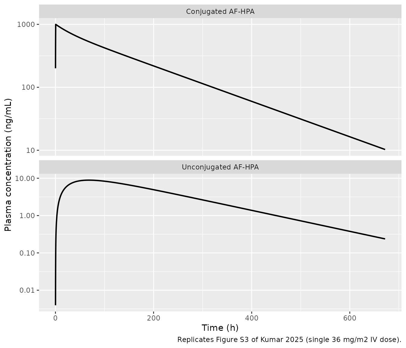
PKNCA validation against Table S3
Table S3 reports the simulated geometric means of AUC from 0 to 28 days, Cmax, the terminal half-life of conjugated AF-HPA and the tmax of unconjugated AF-HPA. A deterministic typical-value curve is compared against those geometric means.
int_28d <- data.frame(start = 0, end = 672, auclast = TRUE, cmax = TRUE,
                      tmax = TRUE, half.life = TRUE)
nca_conj <- run_nca(sim_single, ev_single, "Cc", int_28d)
nca_unconj <- run_nca(sim_single, ev_single, "Cc_afhpa", int_28d)

tbl_conj <- nlmixr2lib::ncaComparisonTable(
  nca_conj,
  data.frame(treatment = "36 mg/m2", auclast = 126902, cmax = 1000, half.life = 107),
  by = "treatment", params = c("auclast", "cmax", "half.life"),
  units = c(auclast = "ng*h/mL", cmax = "ng/mL", half.life = "h")
)
knitr::kable(tbl_conj,
caption = "Conjugated AF-HPA: simulated vs Kumar 2025 Table S3 (simulated geomean). AUC sets the body surface area and the half-life sets the central volume; Cmax is held out.")| NCA parameter | treatment | Reference | Simulated | % diff |
|---|---|---|---|---|
| Cmax (ng/mL) | 36 mg/m2 | 1000 | 999 | -0.1% |
| AUClast (ng*h/mL) | 36 mg/m2 | 127000 | 127000 | +0.2% |
| t½ (h) | 36 mg/m2 | 107 | 106 | -0.7% |
tbl_unconj <- nlmixr2lib::ncaComparisonTable(
  nca_unconj,
  data.frame(treatment = "36 mg/m2", auclast = 2144, cmax = 8.11, tmax = 81.6),
  by = "treatment", params = c("auclast", "cmax", "tmax"),
  units = c(auclast = "ng*h/mL", cmax = "ng/mL", tmax = "h")
)
knitr::kable(tbl_unconj,
caption = "Unconjugated AF-HPA: simulated vs Kumar 2025 Table S3 (simulated geomean AUC and Cmax, median tmax). Nothing here was calibrated.")| NCA parameter | treatment | Reference | Simulated | % diff |
|---|---|---|---|---|
| Cmax (ng/mL) | 36 mg/m2 | 8.11 | 8.89 | +9.6% |
| Tmax (h) | 36 mg/m2 | 81.6 | 68 | -16.7% |
| AUClast (ng*h/mL) | 36 mg/m2 | 2140 | 2120 | -1.2% |
attr(tbl_unconj, "footnote")
#> NULL
v_conj <- nca_values(nca_conj)
v_unconj <- nca_values(nca_unconj)
stopifnot(
  abs(v_conj$cmax / 1000 - 1) < 0.05,      # held-out conjugate Cmax
  abs(v_unconj$auclast / 2144 - 1) < 0.05, # unconjugated AUC0-28d
  abs(v_unconj$cmax / 8.11 - 1) < 0.15     # unconjugated Cmax
)
Conjugated AF-HPA Cmax and unconjugated AF-HPA AUC agree to within a few percent. Unconjugated AF-HPA Cmax is about 10% high and its tmax about 14 h early. Both differences come from collapsing the payload’s whole-body distribution, with its slowly equilibrating tissues, into one compartment. The paper notes that tmax lies in a long sampling gap (48-168 h) and is weakly determined even in the observed data, whose median is 48.4 h.
Multiple dosing: three cycles every 4 weeks (replicates Figure 3 and Table S5)
The cycle-3 lot DAR was 10.6, a conjugated AF-HPA dose of 2.12 mg/m2 (Supplementary Section 3).
ev_md <- make_arm(1L, payload_mg(36, 10.6), c(0, 672, 1344), 2016, "36 mg/m2 q4w")
sim_md <- solve_arms(mod, ev_md)
# Replicates Figure 3 of Kumar 2025 (simulated mean curves only).
sim_md |>
  dplyr::filter(time > 0) |>
  dplyr::select(time, `Conjugated AF-HPA` = Cc, `Unconjugated AF-HPA` = Cc_afhpa) |>
  tidyr::pivot_longer(-time, names_to = "analyte", values_to = "conc") |>
  ggplot(aes(time / 24, conc)) +
  geom_line(linewidth = 0.8) +
  facet_wrap(~analyte, ncol = 1, scales = "free_y") +
  scale_y_log10() +
  labs(x = "Time (days)", y = "Plasma concentration (ng/mL)",
       caption = "Replicates Figure 3 of Kumar 2025 (three 36 mg/m2 IV doses q4w).")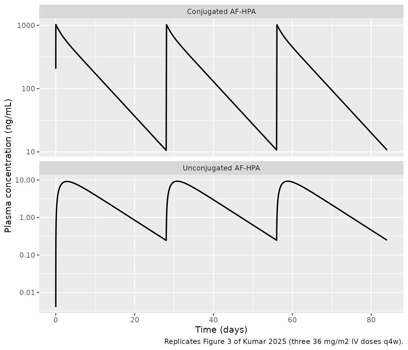
int_c3 <- data.frame(start = 1344, end = 2016, auclast = TRUE, cmax = TRUE)
ref_c3 <- data.frame(
  Analyte = c("Conjugated AF-HPA", "Conjugated AF-HPA",
              "Unconjugated AF-HPA", "Unconjugated AF-HPA"),
  Metric = c("AUC0-28d (ng*h/mL)", "Cmax (ng/mL)", "AUC0-28d (ng*h/mL)", "Cmax (ng/mL)"),
  Published = c(131006, 1047, 2278, 8.57)
)
v_c3_conj <- nca_values(run_nca(sim_md, ev_md, "Cc", int_c3))
v_c3_unconj <- nca_values(run_nca(sim_md, ev_md, "Cc_afhpa", int_c3))
ref_c3$Simulated <- c(v_c3_conj$auclast, v_c3_conj$cmax,
                      v_c3_unconj$auclast, v_c3_unconj$cmax)
ref_c3$`% diff` <- round(100 * (ref_c3$Simulated / ref_c3$Published - 1), 1)
fmt4 <- function(x) vapply(x, function(v) format(signif(v, 4), big.mark = ",", scientific = FALSE, drop0trailing = TRUE), "")
ref_c3$Simulated <- fmt4(ref_c3$Simulated)
fmt_pub <- function(x) vapply(x, function(v) format(v, big.mark = ",", scientific = FALSE, drop0trailing = TRUE), "")
ref_c3$Published <- fmt_pub(ref_c3$Published)
knitr::kable(ref_c3, caption = "Cycle 3 of 36 mg/m2 q4w: simulated vs Kumar 2025 Table S5 (simulated geomean).")| Analyte | Metric | Published | Simulated | % diff |
|---|---|---|---|---|
| Conjugated AF-HPA | AUC0-28d (ng*h/mL) | 131,006 | 131,700 | 0.5 |
| Conjugated AF-HPA | Cmax (ng/mL) | 1,047 | 1,020 | -2.6 |
| Unconjugated AF-HPA | AUC0-28d (ng*h/mL) | 2,278 | 2,217 | -2.7 |
| Unconjugated AF-HPA | Cmax (ng/mL) | 8.57 | 9.303 | 8.6 |
Dose escalation (Table S4)
The dose-escalation lots had no reported DAR, so the paper assumed 10.5 (Supplementary Section 3). The escalation cohorts are separate, small patient groups whose body size differs from the development cohort, so this comparison is looser than the ones above. The model is linear, so it tests dose proportionality and not structure.
doses <- c(20, 30, 36, 43)
ev_esc <- dplyr::bind_rows(lapply(seq_along(doses), function(i) {
  make_arm(i, payload_mg(doses[i], 10.5), 0, 672, paste(doses[i], "mg/m2"))
}))
sim_esc <- solve_arms(mod, ev_esc)
#> Warning: multi-subject simulation without without 'omega'
int_esc <- data.frame(start = 0, end = 672, auclast = TRUE, cmax = TRUE)
v_esc <- dplyr::bind_rows(
  nca_values(run_nca(sim_esc, ev_esc, "Cc", int_esc)) |> dplyr::mutate(Analyte = "Conjugated AF-HPA"),
  nca_values(run_nca(sim_esc, ev_esc, "Cc_afhpa", int_esc)) |> dplyr::mutate(Analyte = "Unconjugated AF-HPA")
)
ref_esc <- data.frame(
  treatment = rep(paste(doses, "mg/m2"), 2),
  Analyte = rep(c("Conjugated AF-HPA", "Unconjugated AF-HPA"), each = 4),
  auc_pub = c(69412, 103129, 118944, 141031, 1039, 1587, 1726, 2383),
  cmax_pub = c(582, 855, 1025, 1151, 4.1, 6.32, 7.16, 9.67)
)
cmp_esc <- dplyr::left_join(ref_esc, v_esc, by = c("treatment", "Analyte")) |>
  dplyr::mutate(
    auc_sim = signif(auclast, 4), auc_pct = round(100 * (auclast / auc_pub - 1), 1),
    cmax_sim = signif(cmax, 3), cmax_pct = round(100 * (cmax / cmax_pub - 1), 1)
  ) |>
  dplyr::select(Analyte, Dose = treatment,
                "AUC0-t published" = auc_pub, "AUC0-t simulated" = auc_sim, "AUC % diff" = auc_pct,
                "Cmax published" = cmax_pub, "Cmax simulated" = cmax_sim, "Cmax % diff" = cmax_pct)
stopifnot(abs(median(c(cmp_esc$`AUC % diff`, cmp_esc$`Cmax % diff`))) < 15)
knitr::kable(dplyr::mutate(cmp_esc, dplyr::across(c(`AUC0-t published`, `Cmax published`), fmt_pub),
                                   dplyr::across(c(`AUC0-t simulated`, `Cmax simulated`), fmt4)),
caption = "Single-dose escalation: simulated vs Kumar 2025 Table S4 (simulated geomean).")| Analyte | Dose | AUC0-t published | AUC0-t simulated | AUC % diff | Cmax published | Cmax simulated | Cmax % diff |
|---|---|---|---|---|---|---|---|
| Conjugated AF-HPA | 20 mg/m2 | 69,412 | 71,990 | 3.7 | 582 | 566 | -2.8 |
| Conjugated AF-HPA | 30 mg/m2 | 103,129 | 108,000 | 4.7 | 855 | 849 | -0.7 |
| Conjugated AF-HPA | 36 mg/m2 | 118,944 | 129,600 | 8.9 | 1,025 | 1,020 | -0.6 |
| Conjugated AF-HPA | 43 mg/m2 | 141,031 | 154,800 | 9.7 | 1,151 | 1,220 | 5.7 |
| Unconjugated AF-HPA | 20 mg/m2 | 1,039 | 1,199 | 15.4 | 4.1 | 5.03 | 22.7 |
| Unconjugated AF-HPA | 30 mg/m2 | 1,587 | 1,799 | 13.4 | 6.32 | 7.55 | 19.4 |
| Unconjugated AF-HPA | 36 mg/m2 | 1,726 | 2,159 | 25.1 | 7.16 | 9.06 | 26.5 |
| Unconjugated AF-HPA | 43 mg/m2 | 2,383 | 2,579 | 8.2 | 9.67 | 10.8 | 11.9 |
Conjugated AF-HPA agrees to within 10% at every dose. Unconjugated AF-HPA runs 8-27% high. Most of that gap reflects the escalation cohorts rather than the reduction. At almost the same 36 mg/m2 dose, the paper’s own simulated unconjugated AUC is 1726 ngh/mL for the escalation cohort (Table S4) and 2144 ngh/mL for the development cohort (Table S3), a 24% difference between virtual cohorts. The reduction is calibrated to the development cohort.
Itraconazole as perpetrator (replicates Table 2)
The itraconazole effect is a multiplicative factor on unconjugated
AF-HPA clearance, set from the published AUC0-inf geometric mean ratio
of the base itraconazole model (CYP3A4 and P-gp both inhibited). The two
single-mechanism scenarios of Table 2 are reproduced by overriding the
factor with 1 / GMR from the same table. The published
Cmax ratios were not used, so reproducing them tests
the reduction’s shape and not only its exposure totals. Conjugated
AF-HPA is unaffected (Table S6, GMR 1.00).
ddi_ratio <- function(factor) {
  ev <- dplyr::bind_rows(
    make_arm(1L, payload_mg(36, 10.0), 0, 3000, "alone"),
    make_arm(2L, payload_mg(36, 10.0), 0, 3000, "itraconazole", itz = 1)
  )
  sim <- rxode2::rxSolve(ui, events = ev, keep = "treatment",
                         params = c(e_itraconazole_cl_afhpa = factor),
                         atol = 1e-10, rtol = 1e-8, returnType = "data.frame")
  v <- nca_values(run_nca(sim, ev, "Cc_afhpa",
                          data.frame(start = 0, end = Inf, aucinf.obs = TRUE, cmax = TRUE)))
  c(auc = v$aucinf.obs[v$treatment == "itraconazole"] / v$aucinf.obs[v$treatment == "alone"],
    cmax = v$cmax[v$treatment == "itraconazole"] / v$cmax[v$treatment == "alone"])
}
scen <- c("Base model (CYP3A4 and P-gp inhibited)" = 1.34,
          "CYP3A4 inhibition only" = 1.02,
          "P-gp inhibition only" = 1.11)
res <- sapply(scen, function(g) ddi_ratio(1 / g))
#> Warning: multi-subject simulation without without 'omega'
#> Warning: multi-subject simulation without without 'omega'
#> Warning: multi-subject simulation without without 'omega'
ddi <- data.frame(
  Scenario = rep(names(scen), each = 2),
  Metric = rep(c("AUC0-inf GMR", "Cmax GMR"), 3),
  Published = c(1.34, 1.21, 1.02, 1.02, 1.11, 1.07),
  Simulated = round(as.vector(res), 3),
  Calibrated = rep(c("yes (sets the CL multiplier)", "no (holdout)"), 3)
)
ddi$`% diff` <- round(100 * (ddi$Simulated / ddi$Published - 1), 1)
knitr::kable(ddi[, c("Scenario", "Metric", "Published", "Simulated", "% diff", "Calibrated")],
caption = "Unconjugated AF-HPA with itraconazole: simulated vs Kumar 2025 Table 2 (geometric mean ratios).")| Scenario | Metric | Published | Simulated | % diff | Calibrated |
|---|---|---|---|---|---|
| Base model (CYP3A4 and P-gp inhibited) | AUC0-inf GMR | 1.34 | 1.340 | 0.0 | yes (sets the CL multiplier) |
| Base model (CYP3A4 and P-gp inhibited) | Cmax GMR | 1.21 | 1.211 | 0.1 | no (holdout) |
| CYP3A4 inhibition only | AUC0-inf GMR | 1.02 | 1.020 | 0.0 | yes (sets the CL multiplier) |
| CYP3A4 inhibition only | Cmax GMR | 1.02 | 1.013 | -0.7 | no (holdout) |
| P-gp inhibition only | AUC0-inf GMR | 1.11 | 1.110 | 0.0 | yes (sets the CL multiplier) |
| P-gp inhibition only | Cmax GMR | 1.07 | 1.072 | 0.2 | no (holdout) |
All three held-out Cmax ratios agree to within about 1%. The Cmax ratio is smaller than the AUC ratio because unconjugated AF-HPA is formation-rate limited: slower payload elimination raises its concentration only gradually, while the conjugate keeps declining. The paper’s ~30% exposure increase with itraconazole therefore carries over to this reduction.
Hepatic impairment (Table 3): not encoded
Kumar 2025 predicted unconjugated AF-HPA AUC0-28d ratios of 1.17, 1.46 and 1.59 and Cmax ratios of 0.98, 1.07 and 1.02 in Child-Pugh A, B and C hepatic impairment versus healthy liver function. These are outputs of Simcyp’s Cirrhosis CP-A/B/C population libraries. Those libraries change hepatic enzyme abundance, liver size and blood flow, plasma albumin (and so fu), haematocrit and renal function together, and the paper prints none of these changes.
The same CL-multiplier encoding that reproduces the itraconazole interaction fails here. The chunk below sets a CL multiplier from each published AUC ratio and checks the held-out Cmax ratio:
hi <- data.frame(
  Class = c("Mild (CP-A)", "Moderate (CP-B)", "Severe (CP-C)"),
  auc_pub = c(1.17, 1.46, 1.59),
  cmax_pub = c(0.98, 1.07, 1.02)
)
hi_res <- sapply(hi$auc_pub, function(g) ddi_ratio(1 / g))
#> Warning: multi-subject simulation without without 'omega'
#> Warning: multi-subject simulation without without 'omega'
#> Warning: multi-subject simulation without without 'omega'
hi$`Cmax GMR, CL multiplier only` <- round(hi_res["cmax", ], 3)
hi$`% diff` <- round(100 * (hi_res["cmax", ] / hi$cmax_pub - 1), 1)
knitr::kable(dplyr::rename(hi, "Published AUC GMR" = auc_pub, "Published Cmax GMR" = cmax_pub),
caption = "A clearance-only encoding of Kumar 2025 Table 3 overpredicts the Cmax ratio in every Child-Pugh class.")| Class | Published AUC GMR | Published Cmax GMR | Cmax GMR, CL multiplier only | % diff |
|---|---|---|---|---|
| Mild (CP-A) | 1.17 | 0.98 | 1.109 | 13.2 |
| Moderate (CP-B) | 1.46 | 1.07 | 1.278 | 19.4 |
| Severe (CP-C) | 1.59 | 1.02 | 1.347 | 32.0 |
A clearance change alone raises the Cmax ratio well above the paper’s near-unity values. The Child-Pugh populations must also change payload distribution or formation, for example through higher fu. Matching both published ratios would need a payload-volume increase of about 40% even in mild impairment, with no value in the paper to support it. The hepatic-impairment scenarios are therefore left out of the model file rather than encoded with parameters calibrated to Table 3. The paper’s observed clinical ratio in mild impairment (AUC 1.01, Cmax 0.96; Table 3) is quoted here for reference.
Assumptions and deviations
- Compartmental reduction. The source is a Simcyp minimal-PBPK plus full-PBPK model. This file reproduces its plasma predictions for the Sim-Cancer population with a 2-compartment conjugate model and a 1-compartment payload model, as derived above. It does not contain the permeability-limited liver, the P-gp efflux kinetics (Jmax 4.80 pmol/min/10^6 cells, KM 10.59 uM), the CYP3A4/CYP3A5 intrinsic clearances, or the CYP3A4 reversible and time-dependent inhibition constants of Table 1. The paper reports these parameters, but they act only through Simcyp physiology it does not print. Payload concentrations, about 10 ng/mL or 12 nM, are three orders of magnitude below the P-gp KM, so the linear reduction loses no saturation.
- Renal-function scaling. The printed renal clearances are read as the healthy-population inputs that Simcyp scales by 0.63 in the Sim-Cancer population (Supplementary Section 12). The scaling cancels out of the unconjugated-to-conjugated AUC ratio checked above. It does set the absolute clearances, and through them the back-solved body surface area. Read the other way, as already-scaled values, the clearances would imply an implausible body surface area of 2.7 m2.
-
Payload release fraction.
fm_afhpa= 0.525 is the recovery-corrected rat fraction, applied to humans as the paper assumes (Model Assumptions). - Body size. The paper reports no body weight, height or body surface area for any cohort. Body surface area (1.71 m2) is back-solved from the conjugated AF-HPA AUC of Table S3, which is why that AUC is not counted as a validation. The payload volume uses a 70 kg reference weight. Between 60 and 72 kg, unconjugated AF-HPA Cmax changes by less than 6%.
- Infusion duration. Not reported. A 30-minute infusion is assumed, which has no visible effect at the 100 h time scale of either analyte.
- Population. The model represents the Sim-Cancer population. The paper’s drug-interaction simulations ran in the healthy-volunteer population, whose absolute payload exposure differs (Table 2: AUC0-inf 1227 ng*h/mL at 2.0 mg/m2). Only the interaction ratios, which the paper reports and which carry over, are reproduced here.
- Itraconazole. The base-model multiplier lumps the CYP3A4 and P-gp mechanisms into one factor. The CYP3A4-only (GMR 1.02) and P-gp-only (GMR 1.11) scenarios do not combine multiplicatively to the base model (1.34), so they are reproduced by overriding the factor, as shown above, rather than as separate parameters.
-
No variability. The paper’s variability is Simcyp
virtual-population physiology, not a random-effects model. The file has
no
etaterms, and its residual errors are fixed at 0.
Results not reproduced by this file
- Hepatic impairment (Table 3): a population-library output; see above.
- Payload as perpetrator (Tables S7 and S8, Figures S4 to S6). The midazolam interaction uses the Simcyp library midazolam model and the Simcyp CYP3A4 turnover (degradation rate constant not printed). The paper predicts a negligible effect (midazolam AUC0-inf GMR 1.04 at a 5-day stagger in cycle 3).
- fmCYP sensitivity analysis (Figure 4): re-partitions the payload clearance among CYP and non-CYP pathways inside the platform. The reduction carries only the total clearance.
- Virtual-population percentiles (Figures 3 and S3, dashed lines): this deterministic reduction produces only the central curve.