Nebulized colistin in ELF and plasma (Lee 2024)
Source:vignettes/articles/Lee_2024_colistin.Rmd
Lee_2024_colistin.RmdModel and source
- Citation: Lee DH, Kim SY, Kim YK, Jung SY, Jang JH, Jang HJ, Lee JH, Jang SM, Lipman J. Intrapulmonary and Systemic Pharmacokinetics of Colistin Following Nebulization of Low-Dose Colistimethate Sodium in Patients with Ventilator-Associated Pneumonia Caused by Carbapenem-Resistant Acinetobacter baumannii. Antibiotics (Basel). 2024;13(3):258. doi:10.3390/antibiotics13030258
- ELF model: One-compartment population PK model with Weibull (time-dependent first-order) absorption for colistin in epithelial lining fluid (ELF) after a 30-min jet nebulization of low-dose colistimethate sodium (CMS) in ventilated adults with ventilator-associated pneumonia caused by carbapenem-resistant Acinetobacter baumannii (Lee 2024). Fit to urea-corrected bronchoalveolar-lavage ELF concentrations only; the companion plasma model is Lee_2024_colistin_plasma. Clearance and volume are apparent (CL/fm, V/fm) and the nebulized dose carries a fixed 9% bioavailability. No covariates.
- Plasma model: One-compartment population PK model with Weibull (time-dependent first-order) absorption for colistin in plasma after a 30-min jet nebulization of low-dose colistimethate sodium (CMS) in ventilated adults with ventilator-associated pneumonia caused by carbapenem-resistant Acinetobacter baumannii (Lee 2024). Fit to plasma concentrations only; the companion epithelial-lining-fluid model is Lee_2024_colistin_elf. Clearance and volume are apparent (CL/fm, V/fm) and the nebulized dose carries a fixed 9% bioavailability. No covariates.
- Article: https://doi.org/10.3390/antibiotics13030258 (open access)
- Supplement (goodness-of-fit plots and VPCs, Figures S1-S4): https://www.mdpi.com/article/10.3390/antibiotics13030258/s1
Lee 2024 fitted two separate population PK models to colistin formed from nebulized colistimethate sodium (CMS): one to epithelial lining fluid (ELF) concentrations and one to plasma concentrations. The two were never linked (CMS itself was not measured), so they are packaged as two independent model files that share this vignette. Both are one-compartment models in which the nebulized dose is absorbed through a Weibull-shaped, time-dependent first-order rate:
where is the time since the start of the current nebulization.
Population
Twenty mechanically ventilated ICU adults (13 male, 7 female; mean age 68.9 years, mean weight 64.9 kg) with ventilator-associated pneumonia caused by carbapenem-resistant Acinetobacter baumannii were enrolled at Haeundae Paik Hospital, Busan, Republic of Korea, between August 2020 and December 2022 (Lee 2024 Table 1). Four were on ECMO and two on CRRT. Each patient received CMS 0.9375 MIU (75 mg CMS, 28.125 mg colistin base activity, CBA) through a jet nebulizer over 30 min every 6 h. ELF was sampled by bronchoalveolar lavage before and 1, 3 and 5 h after the start of a nebulization (80 samples), and plasma before and 1, 2, 3 and 5 h after (100 samples). All pre-dose concentrations were zero (Lee 2024 Figure 1). No covariate was retained.
The same information is available programmatically:
str(readModelDb("Lee_2024_colistin_elf")()$population)
#> List of 12
#>  $ species       : chr "human"
#>  $ n_subjects    : num 20
#>  $ n_studies     : num 1
#>  $ n_observations: num 80
#>  $ age_range     : chr "mean 68.9 years (SD 12.6)"
#>  $ weight_range  : chr "mean 64.9 kg (SD 15.6)"
#>  $ sex_female_pct: num 35
#>  $ race_ethnicity: chr "Korean (single centre, Busan, Republic of Korea)"
#>  $ disease_state : chr "Mechanically ventilated ICU adults with ventilator-associated pneumonia caused by carbapenem-resistant Acinetob"| __truncated__
#>  $ dose_range    : chr "Nebulized CMS 0.9375 MIU (75 mg CMS, 28.125 mg CBA) over 30 min by jet nebulizer every 6 h (3.75 MIU/day)"
#>  $ regions       : chr "Republic of Korea"
#>  $ notes         : chr "Baseline demographics from Lee 2024 Table 1 (13 male / 7 female). 80 ELF concentrations from bronchoalveolar la"| __truncated__
Source trace
Every ini() value carries an in-file comment pointing at
its source. They are collected here.
| Parameter | ELF model | Plasma model | Source |
|---|---|---|---|
lcl (CL/fm) |
log(0.541) mL/min | log(26.3) mL/min | Table 2 |
lvc (V/fm) |
log(23.0) mL | log(67.4) L | Table 2 (V in mL for ELF, L for plasma, per the table footnote) |
lkamax (KAMAX) |
log(0.531) 1/h | log(1.20) 1/h | Table 2 |
lra (RA) |
fixed(log(2.16)) | fixed(log(2.70)) | Table 2, held constant (asterisk) |
lgam1 (GAM) |
fixed(log(2.92)) | fixed(log(1.79)) | Table 2, held constant (asterisk) |
lfdepot (F) |
fixed(log(0.09)) | fixed(log(0.09)) | Section 4.5 and Discussion: bioavailability assumed 9% (Boisson 2014) |
etalcl |
1.24^2 = 1.5376 | 1.96^2 = 3.8416 | Table 2 IIV CL/fm 124% / 196% |
etalvc |
0.597^2 = 0.356409 | 1.11^2 = 1.2321 | Table 2 IIV V/fm 59.7% / 111% |
etalkamax |
0.843^2 = 0.710649 | 0.643^2 = 0.413449 | Table 2 IIV KAMAX 84.3% / 64.3% |
etalra |
fixed(0.83^2) | fixed(0.83^2) | Table 2 IIV RA 83.0%, held constant |
| (IIV on GAM) | none | none | Table 2 IIV GAM 0, held constant |
propSd |
0.271 | 0.185 | Table 2 proportional error 27.1% / 18.5% |
d/dt(depot), d/dt(central)
|
Section 2.3, Eqs. (1) and (3) | ||
Weibull rate wb
|
Section 2.3, Eq. (2) and the Table 2 footnote; see Assumptions |
Units and dosing
Doses are entered in mg of colistin base activity
(CBA) into depot as a 30-min infusion; 1 MIU of CMS = 80 mg
CMS = 30 mg CBA, so the label dose of 75 mg CMS is 28.125 mg CBA. The
model’s fixed bioavailability of 9% applies to that dose. Concentrations
are total colistin in mg/L. Unbound concentrations use the paper’s
assumed unbound fractions: 0.10 in ELF (Gkoufa 2022) and 0.34 in plasma
(Mohamed 2012).
mod_elf <- readModelDb("Lee_2024_colistin_elf")
mod_pla <- readModelDb("Lee_2024_colistin_plasma")
cba_per_mg_cms <- 28.125 / 75
fu <- c(ELF = 0.10, Plasma = 0.34)
Replicate Figure 4: typical-value profiles and steady-state fAUC24
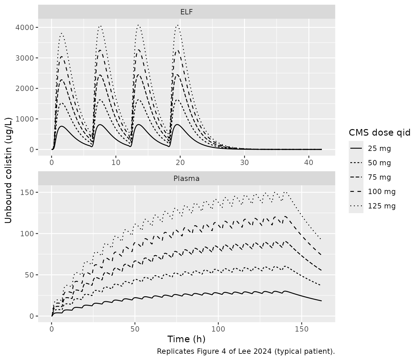
Figure 4 of Lee 2024 shows typical-value unbound profiles for 25 to 125 mg CMS every 6 h, with the steady-state fAUC24 printed in each legend.
doses_cms <- c(25, 50, 75, 100, 125)
fig4_events <- function(dose_cms, n_doses) {
  rxode2::et(
    amt = dose_cms * cba_per_mg_cms, dur = 0.5, ii = 6,
    addl = n_doses - 1, cmt = "depot"
  ) |>
    rxode2::et(seq(0, 6 * n_doses + 18, by = 0.05)) |>
    as.data.frame()
}
sim_fig4 <- function(mod, matrix, n_doses) {
  dplyr::bind_rows(lapply(doses_cms, function(d) {
    s <- rxode2::rxSolve(rxode2::zeroRe(mod), fig4_events(d, n_doses))
    data.frame(time = s$time, Cc = s$Cc, dose = paste(d, "mg"), matrix = matrix)
  }))
}
fig4 <- dplyr::bind_rows(
  sim_fig4(mod_elf, "ELF", 4),
  sim_fig4(mod_pla, "Plasma", 24)
) |>
  dplyr::mutate(
    free_ugL = Cc * 1000 * fu[matrix],
    dose = factor(dose, levels = paste(doses_cms, "mg"))
  )
#> ℹ parameter labels from comments will be replaced by 'label()'
#> ℹ omega/sigma items treated as zero: 'etalcl', 'etalvc', 'etalkamax', 'etalra'
#> ℹ parameter labels from comments will be replaced by 'label()'
#> ℹ omega/sigma items treated as zero: 'etalcl', 'etalvc', 'etalkamax', 'etalra'
#> ℹ parameter labels from comments will be replaced by 'label()'
#> ℹ omega/sigma items treated as zero: 'etalcl', 'etalvc', 'etalkamax', 'etalra'
#> ℹ parameter labels from comments will be replaced by 'label()'
#> ℹ omega/sigma items treated as zero: 'etalcl', 'etalvc', 'etalkamax', 'etalra'
#> ℹ parameter labels from comments will be replaced by 'label()'
#> ℹ omega/sigma items treated as zero: 'etalcl', 'etalvc', 'etalkamax', 'etalra'
#> ℹ parameter labels from comments will be replaced by 'label()'
#> ℹ omega/sigma items treated as zero: 'etalcl', 'etalvc', 'etalkamax', 'etalra'
#> ℹ parameter labels from comments will be replaced by 'label()'
#> ℹ omega/sigma items treated as zero: 'etalcl', 'etalvc', 'etalkamax', 'etalra'
#> ℹ parameter labels from comments will be replaced by 'label()'
#> ℹ omega/sigma items treated as zero: 'etalcl', 'etalvc', 'etalkamax', 'etalra'
#> ℹ parameter labels from comments will be replaced by 'label()'
#> ℹ omega/sigma items treated as zero: 'etalcl', 'etalvc', 'etalkamax', 'etalra'
#> ℹ parameter labels from comments will be replaced by 'label()'
#> ℹ omega/sigma items treated as zero: 'etalcl', 'etalvc', 'etalkamax', 'etalra'
ggplot(fig4, aes(time, free_ugL, linetype = dose)) +
  geom_line() +
  facet_wrap(~matrix, ncol = 1, scales = "free") +
  labs(
    x = "Time (h)", y = "Unbound colistin (ug/L)", linetype = "CMS dose qid",
    caption = "Replicates Figure 4 of Lee 2024 (typical patient)."
  )
The steady-state fAUC24 is four times the unbound AUC over the last
6-h interval of 80 doses (20 days, about 16 plasma half-lives, so the
residual approach to steady state is below 0.01%). An
ss = 1 steady-state dose is not used here: with the
time-after-dose Weibull rate it settled about 0.9% low for ELF.
fauc_ss <- function(mod, matrix, dose_cms, n_doses = 80) {
  t_last <- 6 * (n_doses - 1)
  ev <- rxode2::et(
    amt = dose_cms * cba_per_mg_cms, dur = 0.5, ii = 6, addl = n_doses - 1,
    cmt = "depot"
  ) |>
    rxode2::et(seq(t_last, t_last + 6, by = 0.01))
  s <- as.data.frame(rxode2::rxSolve(
    rxode2::zeroRe(mod), ev,
    rtol = 1e-10, atol = 1e-12, maxsteps = 1e6
  ))
  cf <- s$Cc * 1000 * fu[[matrix]]
  4 * sum(diff(s$time) * (head(cf, -1) + tail(cf, -1)) / 2)
}
published_fauc <- tibble::tribble(
  ~matrix, ~dose_cms, ~published,
  "ELF", 125, 51987, "ELF", 100, 41590, "ELF", 75, 31192, "ELF", 50, 20795,
  "ELF", 25, 10397,
  "Plasma", 125, 3636, "Plasma", 100, 2909, "Plasma", 75, 2182,
  "Plasma", 50, 1454, "Plasma", 25, 727
)
fauc_tab <- published_fauc |>
  dplyr::rowwise() |>
  dplyr::mutate(
    simulated = fauc_ss(
      if (matrix == "ELF") mod_elf else mod_pla, matrix, dose_cms
    )
  ) |>
  dplyr::ungroup() |>
  dplyr::mutate(pct_diff = 100 * (simulated / published - 1))
#> ℹ parameter labels from comments will be replaced by 'label()'
#> ℹ omega/sigma items treated as zero: 'etalcl', 'etalvc', 'etalkamax', 'etalra'
#> ℹ parameter labels from comments will be replaced by 'label()'
#> ℹ omega/sigma items treated as zero: 'etalcl', 'etalvc', 'etalkamax', 'etalra'
#> ℹ parameter labels from comments will be replaced by 'label()'
#> ℹ omega/sigma items treated as zero: 'etalcl', 'etalvc', 'etalkamax', 'etalra'
#> ℹ parameter labels from comments will be replaced by 'label()'
#> ℹ omega/sigma items treated as zero: 'etalcl', 'etalvc', 'etalkamax', 'etalra'
#> ℹ parameter labels from comments will be replaced by 'label()'
#> ℹ omega/sigma items treated as zero: 'etalcl', 'etalvc', 'etalkamax', 'etalra'
#> ℹ parameter labels from comments will be replaced by 'label()'
#> ℹ omega/sigma items treated as zero: 'etalcl', 'etalvc', 'etalkamax', 'etalra'
#> ℹ parameter labels from comments will be replaced by 'label()'
#> ℹ omega/sigma items treated as zero: 'etalcl', 'etalvc', 'etalkamax', 'etalra'
#> ℹ parameter labels from comments will be replaced by 'label()'
#> ℹ omega/sigma items treated as zero: 'etalcl', 'etalvc', 'etalkamax', 'etalra'
#> ℹ parameter labels from comments will be replaced by 'label()'
#> ℹ omega/sigma items treated as zero: 'etalcl', 'etalvc', 'etalkamax', 'etalra'
#> ℹ parameter labels from comments will be replaced by 'label()'
#> ℹ omega/sigma items treated as zero: 'etalcl', 'etalvc', 'etalkamax', 'etalra'
fauc_tab |>
  dplyr::mutate(simulated = round(simulated), pct_diff = round(pct_diff, 2)) |>
  dplyr::rename(
    "Matrix" = matrix, "CMS dose qid (mg)" = dose_cms,
    "Published fAUC24 (ug*h/L)" = published,
    "Simulated fAUC24 (ug*h/L)" = simulated, "Difference (%)" = pct_diff
  ) |>
knitr::kable(caption = "Steady-state fAUC24, simulated vs Lee 2024 Figure 4.")| Matrix | CMS dose qid (mg) | Published fAUC24 (ug*h/L) | Simulated fAUC24 (ug*h/L) | Difference (%) |
|---|---|---|---|---|
| ELF | 125 | 51987 | 51987 | 0.00 |
| ELF | 100 | 41590 | 41590 | 0.00 |
| ELF | 75 | 31192 | 31192 | 0.00 |
| ELF | 50 | 20795 | 20795 | 0.00 |
| ELF | 25 | 10397 | 10397 | 0.00 |
| Plasma | 125 | 3636 | 3636 | 0.00 |
| Plasma | 100 | 2909 | 2909 | -0.01 |
| Plasma | 75 | 2182 | 2182 | -0.02 |
| Plasma | 50 | 1454 | 1454 | 0.02 |
| Plasma | 25 | 727 | 727 | 0.02 |
# Deterministic: a typical-value solve against the paper's own typical-value
# numbers. The paper rounds to the unit, so agreement is to well under 0.5%;
# a dose-unit error (CMS instead of CBA) or a dropped bioavailability moves
# every row by a factor of 2.7 or 11.
stopifnot(max(abs(fauc_tab$pct_diff)) < 0.5)
The agreement pins three conventions at once: the dose is CBA, the 9% bioavailability sits inside the model, and the unbound fractions are 0.10 (ELF) and 0.34 (plasma).
The first-dose ELF peak also identifies the form of the Weibull function (see Assumptions). Digitised from Figure 4a, the 125 mg first-dose peak is about 3,800 ug/L unbound at about 1.55 h after the start of nebulization.
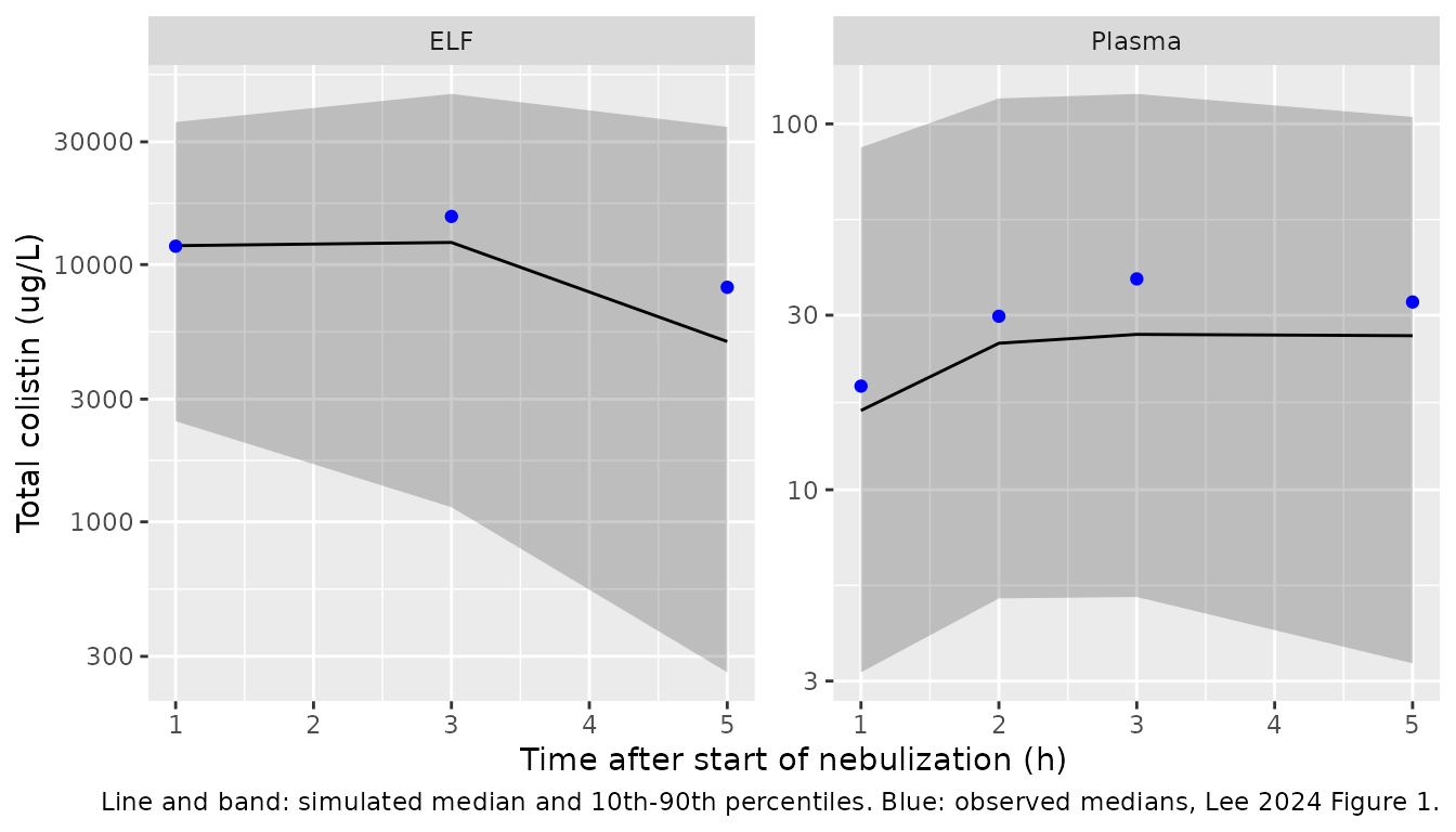
Replicate Figure 1 and the supplementary VPCs (Figures S3 and S4)
The study design (one 28.125 mg CBA dose over 30 min; ELF sampled at 1, 3 and 5 h; plasma at 1, 2, 3 and 5 h) is simulated with between-subject and residual variability for 200 virtual patients per matrix.
rxode2::rxSetSeed(20240314)
n_sub <- 200
vpc_events <- function(obs_times) {
  dose <- data.frame(
    id = seq_len(n_sub), time = 0, amt = 28.125, dur = 0.5, evid = 1,
    cmt = "depot"
  )
  obs <- tidyr::expand_grid(id = seq_len(n_sub), time = c(0, obs_times)) |>
    dplyr::mutate(amt = NA_real_, dur = NA_real_, evid = 0, cmt = "central")
  dplyr::bind_rows(dose, obs) |> dplyr::arrange(id, time, dplyr::desc(evid))
}
vpc_elf <- rxode2::rxSolve(mod_elf, vpc_events(c(1, 3, 5))) |>
  as.data.frame() |>
  dplyr::mutate(matrix = "ELF")
#> ℹ parameter labels from comments will be replaced by 'label()'
vpc_pla <- rxode2::rxSolve(mod_pla, vpc_events(c(1, 2, 3, 5))) |>
  as.data.frame() |>
  dplyr::mutate(matrix = "Plasma")
#> ℹ parameter labels from comments will be replaced by 'label()'
# Pre-dose (time 0) rows are kept for PKNCA below and left out of the
# percentile summaries.
vpc <- dplyr::bind_rows(vpc_elf, vpc_pla) |>
  dplyr::mutate(dv_ugL = sim * 1000)

vpc_q <- vpc |>
  dplyr::filter(time %in% c(1, 2, 3, 5)) |>
  dplyr::group_by(matrix, time) |>
  dplyr::summarise(
    p10 = quantile(dv_ugL, 0.10), p50 = median(dv_ugL),
    p90 = quantile(dv_ugL, 0.90), .groups = "drop"
  )
observed_median <- tibble::tribble(
  ~matrix, ~time, ~obs_median,
  "ELF", 1, 11790, "ELF", 3, 15386, "ELF", 5, 8164,
  "Plasma", 1, 19.2, "Plasma", 2, 29.8, "Plasma", 3, 37.7, "Plasma", 5, 32.6
)
ggplot(vpc_q, aes(time)) +
  geom_ribbon(aes(ymin = p10, ymax = p90), alpha = 0.25) +
  geom_line(aes(y = p50)) +
  geom_point(aes(y = obs_median), data = observed_median, colour = "blue") +
  facet_wrap(~matrix, scales = "free_y") +
  scale_y_log10() +
  labs(
    x = "Time after start of nebulization (h)", y = "Total colistin (ug/L)",
    caption = paste(
      "Line and band: simulated median and 10th-90th percentiles.",
      "Blue: observed medians, Lee 2024 Figure 1."
    )
  )
# Simulated 10th / 50th / 90th percentiles digitised by the maintainers from
# the dashed lines of Figures S3b and S4b (semi-log panels).
digitised <- tibble::tribble(
  ~matrix, ~time, ~vpc_p10, ~vpc_p50, ~vpc_p90,
  "ELF", 1, 1580, 10500, 41100,
  "ELF", 3, 1300, 10500, 48500,
  "Plasma", 1, 2.1, 16.3, 108,
  "Plasma", 3, 3.6, 25.4, 142,
  "Plasma", 5, 2.3, 23.5, 134
)
cmp_vpc <- vpc_q |>
  dplyr::left_join(observed_median, by = c("matrix", "time")) |>
  dplyr::left_join(digitised, by = c("matrix", "time"))
cmp_vpc |>
  dplyr::mutate(dplyr::across(c(p10, p50, p90), ~ signif(.x, 3))) |>
  dplyr::rename(
    "Matrix" = matrix, "Time (h)" = time,
    "Sim P10" = p10, "Sim median" = p50, "Sim P90" = p90,
    "Observed median (Fig. 1)" = obs_median,
    "VPC P10 (Fig. S3/S4)" = vpc_p10, "VPC median (Fig. S3/S4)" = vpc_p50,
    "VPC P90 (Fig. S3/S4)" = vpc_p90
  ) |>
knitr::kable(caption = "Simulated percentiles (ug/L) against Lee 2024.")| Matrix | Time (h) | Sim P10 | Sim median | Sim P90 | Observed median (Fig. 1) | VPC P10 (Fig. S3/S4) | VPC median (Fig. S3/S4) | VPC P90 (Fig. S3/S4) |
|---|---|---|---|---|---|---|---|---|
| ELF | 1 | 2460.00 | 11800.0 | 35800.0 | 11790.0 | 1580.0 | 10500.0 | 41100 |
| ELF | 3 | 1140.00 | 12200.0 | 46100.0 | 15386.0 | 1300.0 | 10500.0 | 48500 |
| ELF | 5 | 260.00 | 5020.0 | 34300.0 | 8164.0 | NA | NA | NA |
| Plasma | 1 | 3.17 | 16.5 | 86.2 | 19.2 | 2.1 | 16.3 | 108 |
| Plasma | 2 | 5.05 | 25.1 | 117.0 | 29.8 | NA | NA | NA |
| Plasma | 3 | 5.09 | 26.6 | 121.0 | 37.7 | 3.6 | 25.4 | 142 |
| Plasma | 5 | 3.35 | 26.4 | 105.0 | 32.6 | 2.3 | 23.5 | 134 |
# Centre of a 200-subject cohort against the observed medians of 20 patients.
# On a 20,000-subject cohort the simulated/observed median ratios are
# 0.64-0.91 (geometric mean about 0.74). The between-subject SD of log
# concentration is 1.0-1.9, so a 200-subject median carries a log-scale SE of
# 0.1-0.17 per point: a per-point factor-of-2 bound would sit only 1.5 SE from
# the ELF 5 h ratio. The gate is therefore on the geometric mean of the seven
# ratios (bound 0.5-1.5, more than 3 SE either side), plus a factor-of-3
# envelope per point. A dose-unit error (2.7-fold) or a dropped bioavailability
# (11-fold) moves the geometric mean outside 0.5-1.5. Over six seeds and
# 1/2/4 solver threads the realised geometric mean was 0.72-0.85 and the
# smallest single ratio 0.60.
ratio <- cmp_vpc$p50 / cmp_vpc$obs_median
stopifnot(
  exp(mean(log(ratio))) > 0.5, exp(mean(log(ratio))) < 1.5,
  all(ratio > 1 / 3 & ratio < 3)
)
The simulated medians sit 10-35% below the observed medians, as the authors’ own VPC medians do (Figures S3 and S4: 10,500 against an observed 15,386 ug/L in ELF at 3 h). With 200 virtual patients the 10th and 90th percentiles are themselves noisy (roughly +/-30% between draws), so they are shown for orientation; the comparison of the IIV readings against these VPC percentiles was made on a 20,000-subject cohort (see Assumptions). For plasma the authors’ simulated 90th percentile sits somewhat above the packaged model’s under either reading.
Replicate Table 3: individual steady-state fAUC24
Lee 2024 computed each patient’s steady-state fAUC24 for 75 mg CMS every 6 h as F x fu x daily dose / CL, using the post-hoc CL. The virtual cohort below uses the same formula on simulated individual clearances.
fauc_ind <- dplyr::bind_rows(vpc_elf, vpc_pla) |>
  dplyr::distinct(id, matrix, cl) |>
  dplyr::mutate(fauc_mgh_L = 0.09 * fu[matrix] * 4 * 28.125 / cl) |>
  dplyr::group_by(matrix) |>
  dplyr::summarise(
    median = median(fauc_mgh_L), q25 = quantile(fauc_mgh_L, 0.25),
    q75 = quantile(fauc_mgh_L, 0.75), .groups = "drop"
  )
fauc_ind |>
  dplyr::mutate(dplyr::across(c(median, q25, q75), ~ signif(.x, 3))) |>
  dplyr::rename(
    "Matrix" = matrix, "Median (mg*h/L)" = median, "Q1" = q25, "Q3" = q75
  ) |>
  knitr::kable(caption = paste(
    "Simulated fAUC24. Lee 2024 Table 3 medians by clinical outcome:",
    "ELF 36.7 (cured) and 31.7 (failed); plasma 1.40 and 2.00 mg*h/L."
))| Matrix | Median (mg*h/L) | Q1 | Q3 |
|---|---|---|---|
| ELF | 34.20 | 13.000 | 69.40 |
| Plasma | 2.45 | 0.567 | 6.93 |
The simulated interquartile ranges are wider than the published ones because the published values are post-hoc estimates, which shrink toward the typical value when each patient contributes only three or four samples.
PKNCA validation
PKNCA is run on the simulated observations at the study sampling times (with residual error), per matrix, and compared against the observed median (IQR) peak concentrations quoted in the Discussion: 21,950 (10,440-28,389) ug/L in ELF and 43.51 (14.23-85.78) ug/L in plasma.
# Subjects drawn with a very high clearance decay to numerically zero by 5 h,
# where the integrator can undershoot by about its absolute tolerance. Check it
# is noise, then floor it so PKNCA sees no negative concentration.
stopifnot(all(vpc$dv_ugL >= -1e-6 * max(vpc$dv_ugL), na.rm = TRUE))
nca_conc <- vpc |>
  dplyr::filter(!is.na(dv_ugL)) |>
  dplyr::transmute(id, treatment = matrix, time, Cc = pmax(dv_ugL, 0)) |>
  dplyr::arrange(treatment, id, time)
nca_dose <- dplyr::distinct(nca_conc, id, treatment) |>
  dplyr::mutate(time = 0, amt = 28.125)

conc_obj <- PKNCA::PKNCAconc(nca_conc, Cc ~ time | treatment + id)
dose_obj <- PKNCA::PKNCAdose(nca_dose, amt ~ time | treatment + id)
intervals <- data.frame(start = 0, end = 5, cmax = TRUE, tmax = TRUE, auclast = TRUE)
nca_res <- PKNCA::pk.nca(PKNCA::PKNCAdata(conc_obj, dose_obj, intervals = intervals))

published_nca <- tibble::tribble(
  ~treatment, ~cmax,
  "ELF", 21950,
  "Plasma", 43.51
)
cmp <- nlmixr2lib::ncaComparisonTable(
  simulated = nca_res,
  reference = published_nca,
  by = "treatment",
  units = c(cmax = "ug/L", tmax = "h", auclast = "ug*h/L"),
  tolerance_pct = 20
)
knitr::kable(
  cmp,
  caption = paste(
    "Simulated vs. observed median peak concentration (single 75 mg CMS",
    "nebulization). * differs from the reference by more than 20%."
  )
)| NCA parameter | treatment | Reference | Simulated | % diff |
|---|---|---|---|---|
| Cmax (ug/L) | ELF | 22000 | 18800 | -14.4% |
| Cmax (ug/L) | Plasma | 43.5 | 34.8 | -20.0%* |
cmax_med <- as.data.frame(nca_res) |>
  dplyr::filter(PPTESTCD == "cmax") |>
  dplyr::group_by(treatment) |>
  dplyr::summarise(med = median(PPORRES), .groups = "drop") |>
  dplyr::left_join(published_nca, by = "treatment")
cmax_med
#> # A tibble: 2 × 3
#>   treatment     med    cmax
#>   <chr>       <dbl>   <dbl>
#> 1 ELF       18787.  21950
#> 2 Plasma       34.8    43.5
# Factor-of-2 envelope: the realised ratio over six seeds was 0.86-0.94 (ELF)
# and 0.69-0.80 (plasma); a dose-unit or bioavailability error moves it
# 2.7- to 11-fold.
stopifnot(all(cmax_med$med / cmax_med$cmax > 0.5 & cmax_med$med / cmax_med$cmax < 2))
The simulated median peaks sit roughly 5-30% below the observed medians in both matrices (over six seeds the ratio was 0.86-0.94 for ELF and 0.69-0.80 for plasma, so the plasma row is usually flagged at the 20% line). The reference is the median of only 20 observed peaks, and the typical model curves already sit slightly below the observed medians at 3 h in Figure 1 (ELF 15.2 vs 15.4 mg/L; plasma 34 vs 38 ug/L), so this is read as sampling noise in the reference rather than a transcription error, which would move the peak several-fold.
Assumptions and deviations
-
Form of the Weibull function. Lee 2024 prints Eq.
(2) in MathML as
KAMAX x (1 - (exp(-RA x time))^GAM)and the Table 2 footnote asKAMAX x (1 - exp(-RA x time)^GAM). Read literally,(exp(-RA t))^GAMequalsexp(-RA GAM t), in which RA and GAM collapse into one rate constant, which would make two separately reported, separately fixed parameters meaningless. The packaged models use the standard Weibull formKAMAX x (1 - exp(-(RA x t)^GAM))of the isavuconazole model the paper cites for it (Desai 2016, ref. 15; packaged asDesai_2016_isavuconazole_secure). The maintainers checked all three readings against Figure 4a: the standard form puts the first-dose ELF peak at 1.55 h, matching the figure; the literal form puts it at 1.30 h, and(1 - exp(-RA t))^GAMlowers the peak by 8% (to about 3,490 ug/L for 125 mg, against about 3,800 in the figure).tis the time since the start of the current nebulization (tad(depot)), which reproduces the identical repeated peaks of Figure 4a. - Bioavailability. The paper says the 9% bioavailability (Boisson 2014) was assumed “to calculate the PK/PD index”. It is inside the fitted model as well: the Figure 4 typical-value curves (and fAUC24 values) are reproduced exactly with F = 0.09, and these typical curves match the observed Figure 1 medians. With F = 1 every prediction would be 11-fold too high.
- Dose units. The models take the dose in mg CBA. Figure 4 labels doses in mg CMS; the fAUC24 agreement above (which is exact only for CBA) pins the conversion 75 mg CMS = 28.125 mg CBA given in the Figure 1 caption.
- Nebulization as a 30-min infusion into the depot. The paper does not say how the 30-min nebulization was coded. Modelling it as a bolus into the depot changes the ELF peak by less than 1% and its timing by less than 0.1 h, because the Weibull rate is still below a fifth of KAMAX at 15 min.
-
IIV scale. Table 2 gives IIV as percentages under
theta_i = theta x exp(eta_i)without saying how they were computed. The maintainers read them assqrt(omega^2) x 100(the PsN convention; PsN was used for the bootstrap), givingomega^2 = (pct/100)^2. The alternativeomega^2 = log(1 + CV^2)gives markedly smaller variances for these large values (e.g. 1.58 instead of 3.84 for plasma CL). The maintainers simulated both readings (20,000 subjects each, with residual error) against the digitised dashed percentile lines of the supplementary VPCs: at 1 h in ELF the chosen reading gives 1,600 / 10,700 / 41,700 ug/L against 1,580 / about 10,500 / 41,100 digitised, whilelog(1 + CV^2)gives 2,530 / 12,000 / 38,100. - IIV on GAM is reported as 0 (held constant) and the packaged models carry no eta on it. IIV on RA is held at 83.0% in both models, as published.
- Unbound concentrations are not model outputs. The unbound fractions 0.10 (ELF) and 0.34 (plasma) are the paper’s assumptions and are applied in this vignette only.
-
CL and V units. The
ini()values keep the paper’s units (CL in mL/min; V in mL for ELF and L for plasma);model()converts to L/h and L. - No correction notice for Lee 2024 was found as of 2026-10-29.