Vancomycin (Kirwan 2021)
Source:vignettes/articles/Kirwan_2021_vancomycin.Rmd
Kirwan_2021_vancomycin.RmdModel and source
mod <- readModelDb("Kirwan_2021_vancomycin")
ui <- rxode2::rxode(mod)- Citation: Kirwan M, Munshi R, O’Keeffe H, Judge C, Coyle M, Deasy E, Kelly YP, Lavin PJ, Donnelly M, D’Arcy DM. Exploring population pharmacokinetic models in patients treated with vancomycin during continuous venovenous haemodiafiltration (CVVHDF). Crit Care. 2021;25(1):443. doi:10.1186/s13054-021-03863-4. PMCID: PMC8691013.
- Description: One-compartment intravenous population PK model for vancomycin given by intermittent infusion to critically ill adults receiving continuous venovenous haemodiafiltration (CVVHDF) in a single Irish tertiary ICU. Fitted non-parametrically with the NPAG algorithm in Pmetrics to peak and trough therapeutic-drug-monitoring levels only. Clearance (total, i.e. residual native plus CVVHDF) and volume of distribution carry inter-individual variability; no covariate was retained – the base structural model is the final model, and it is the model the authors used for their probability-of-target-attainment dosing simulations. Residual unexplained variability is carried as fixed(0) because the Pmetrics assay-error polynomial and the fitted gamma/lambda term were never published.
- Article: https://doi.org/10.1186/s13054-021-03863-4 (open access, CC BY 4.0)
- Supplement (Additional file 1, Tables S1-S2 and Figures S1-S2): available from the article page.
Kirwan and colleagues fitted a one-compartment model to routine peak and trough therapeutic-drug-monitoring (TDM) levels with the non-parametric adaptive grid (NPAG) algorithm in Pmetrics. They screened a long list of continuous and categorical covariates, found that none gave a clear improvement, and used the base structural model – clearance and volume only – for their probability-of-target-attainment (PTA) dosing simulations. That base model is the model packaged here.
Population
The analysis used 106 vancomycin dosing intervals from 24 critically ill adults in a single tertiary intensive care unit in Dublin, Ireland, all receiving continuous venovenous haemodiafiltration (CVVHDF) for most of each included dosing interval (Methods; Table 1). Eighteen of 24 (75%) were male; mean age was 65.5 years (SD 12.3), mean weight 81.8 kg (SD 24), mean BMI 28.6 kg/m^2. Patients were severely ill (APACHE II mean 23, SOFA mean 10.5, in-hospital mortality 25%) and largely anuric (median urine output on study day 1, 77.9 mL/24 h). The ICU dosing policy was a 25 mg/kg loading dose followed by 15-20 mg/kg once daily, infused at 10 mg/min; the doses actually recorded averaged 1098 mg (SD 249) at a mean interval of 18.5 h (Table 2). Peaks were drawn 60 min after the end of the infusion and troughs immediately before the next dose.
str(ui$population[c("n_subjects", "n_dosing_intervals", "sex_female_pct",
                    "age_range", "weight_range", "regions")])
#> List of 6
#>  $ n_subjects        : int 24
#>  $ n_dosing_intervals: int 106
#>  $ sex_female_pct    : num 25
#>  $ age_range         : chr "mean 65.5 (SD 12.3) years; median 67 (IQR 56.8-75.3)"
#>  $ weight_range      : chr "mean 81.8 (SD 24) kg; median 79.9 (IQR 61.3-91.5)"
#>  $ regions           : chr "Ireland (Tallaght University Hospital, Dublin; single centre)"
Source trace
Every value below is also carried as an in-file comment next to its
ini() entry in
inst/modeldb/specificDrugs/Kirwan_2021_vancomycin.R.
| Model element | Value | Source location |
|---|---|---|
| Structural model | 1-compartment, IV infusion, first-order elimination | Methods, ‘Population pharmacokinetic analysis’ |
lcl (total CL on CVVHDF) |
log(2.59 L/h) | Table 3, base model CL mean (SD 0.49, CV 18.99%, median 2.70); Results text |
lvc (V) |
log(80.98 L) | Table 3, base model V mean (SD 16.89, CV 20.86%, median 73.72); Results text |
etalcl |
0.035427 = log(0.1899^2 + 1) | Table 3, base model CL CV% |
etalvc |
0.042594 = log(0.2086^2 + 1) | Table 3, base model V CV% |
addSd, propSd
|
fixed(0) | Not reported (see Assumptions and deviations) |
d/dt(central) <- -kel * central,
Cc <- central / vc
|
n/a | Methods, ‘Population pharmacokinetic analysis’ |
| Infusion rate 10 mg/min | n/a | Methods, ‘Vancomycin therapy and TDM’ |
| PTA regimens 1-4 | n/a | Methods, ‘Probability of target attainment (PTA) plots’; Figure 2; Additional file 1 Figures S1-S2 |
Virtual cohort
Original observed data are not publicly available. The final model has no covariates, so a virtual subject is defined by its dosing regimen alone. The cohort simulates the four exploratory regimens of the paper’s PTA analysis (Methods), with 200 virtual patients per regimen (the paper used 1000):
- 2 g loading dose, then 750 mg every 12 h from 12 h;
- 2 g loading dose, then 500 mg every 12 h from 12 h;
- 1.5 g loading dose, then 750 mg every 12 h from 12 h;
- 2 g loading dose, then 1.5 g at 12 h and 1.5 g every 24 h thereafter.
Every dose is infused at the ICU’s 10 mg/min (600 mg/h). Observations
run on a 0.25-h grid to 48 h on the central state; because
the doses are infusions, the concentration at a dose time equals the
pre-dose (trough) value.
regimens <- list(
  "R1: 2 g then 750 mg q12h" = data.frame(time = c(0, 12, 24, 36), amt = c(2000, 750, 750, 750)),
  "R2: 2 g then 500 mg q12h" = data.frame(time = c(0, 12, 24, 36), amt = c(2000, 500, 500, 500)),
  "R3: 1.5 g then 750 mg q12h" = data.frame(time = c(0, 12, 24, 36), amt = c(1500, 750, 750, 750)),
  "R4: 2 g, 1.5 g at 12 h, then q24h" = data.frame(time = c(0, 12, 36), amt = c(2000, 1500, 1500))
)
n_per_regimen <- 200L
obs_times <- seq(0, 48, by = 0.25)

make_cohort <- function(regimen, doses, n, id_offset) {
  ids <- id_offset + seq_len(n)
  dose_rows <- tidyr::expand_grid(id = ids, doses) |>
    dplyr::mutate(evid = 1L, cmt = "central", rate = 600)
  obs_rows <- tidyr::expand_grid(id = ids, time = obs_times) |>
    dplyr::mutate(evid = 0L, amt = NA_real_, cmt = "central", rate = NA_real_)
  dplyr::bind_rows(dose_rows, obs_rows) |>
    dplyr::mutate(regimen = regimen) |>
    dplyr::arrange(id, time, dplyr::desc(evid))
}

events <- dplyr::bind_rows(lapply(seq_along(regimens), function(i) {
  make_cohort(names(regimens)[i], regimens[[i]], n_per_regimen,
              id_offset = (i - 1L) * n_per_regimen)
}))
stopifnot(!anyDuplicated(unique(events[, c("id", "time", "evid")])))
Simulation
rxode2::rxSetSeed(20211210)
sim <- rxode2::rxSolve(mod, events = events, keep = "regimen") |>
  as.data.frame()
Typical-value check against the closed form
With the random effects zeroed, the one-compartment infusion model has a closed-form superposition solution. Both sides use the same parameters, so the difference is pure numerical error and a tight bound is appropriate.
sim_typ <- rxode2::rxSolve(rxode2::zeroRe(mod),
                           events = dplyr::filter(events, id == 1L)) |>
  as.data.frame()
#> ℹ omega/sigma items treated as zero: 'etalcl', 'etalvc'

cl <- 2.59; v <- 80.98; k <- cl / v
closed_form <- function(t, doses, rate = 600) {
  vapply(t, function(tt) {
    sum(vapply(seq_len(nrow(doses)), function(j) {
      dur <- doses$amt[j] / rate
      ts <- tt - doses$time[j]
      if (ts <= 0) return(0)
      r0 <- rate / cl
      if (ts <= dur) r0 * (1 - exp(-k * ts))
      else r0 * (1 - exp(-k * dur)) * exp(-k * (ts - dur))
    }, numeric(1)))
  }, numeric(1))
}
cf <- closed_form(sim_typ$time, regimens[[1]])
stopifnot(max(abs(sim_typ$Cc - cf) / pmax(cf, 1)) < 1e-4)
The typical patient on regimen 1 has a trough of 17.8 mg/L at 12 h and 19.4 mg/L at 48 h; the elimination half-life is 21.7 h.
sim |>
  dplyr::group_by(regimen, time) |>
  dplyr::summarise(
    Q05 = quantile(Cc, 0.05), Q50 = median(Cc), Q95 = quantile(Cc, 0.95),
    .groups = "drop"
  ) |>
  ggplot(aes(time, Q50)) +
  geom_ribbon(aes(ymin = Q05, ymax = Q95), alpha = 0.25) +
  geom_line() +
  geom_hline(yintercept = c(15, 20), linetype = "dashed", colour = "grey40") +
  facet_wrap(~regimen) +
  scale_x_continuous(breaks = seq(0, 48, 12)) +
  labs(x = "Time after first dose (h)", y = "Vancomycin Cc (mg/L)")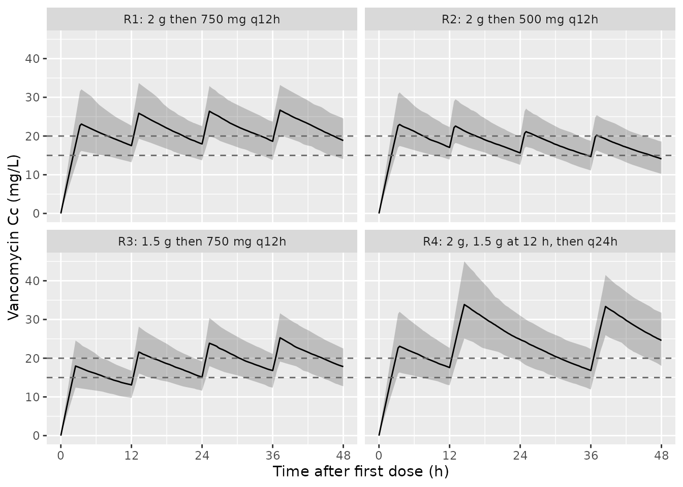
Simulated vancomycin concentration by regimen: median and 5th-95th percentiles over the first 48 h (200 virtual patients per regimen).
Replicate Figure 2 (trough PTA)
Figure 2 of Kirwan 2021 plots, for each regimen, the proportion of simulated patients whose pre-dose concentration at 12, 24, 36 and 48 h reaches 10, 15, 18, 20 and 25 mg/L. The published points below were digitised by the maintainers from the high-resolution Figure 2 raster (reading resolution about +/-0.02). At 12 h the three 2 g-loading regimens are the same regimen; the black regimen-1 line is hidden under the other two and was not digitised. Regimen 4 has no trough at 24 or 48 h.
fig2_pub <- tibble::tribble(
  ~regimen_short, ~time, ~conc, ~prop_pub,
  "R2", 12, 15, 0.86, "R2", 12, 18, 0.43, "R2", 12, 20, 0.17,
  "R4", 12, 15, 0.82, "R4", 12, 18, 0.37, "R4", 12, 20, 0.13,
  "R3", 12, 15, 0.11, "R3", 12, 18, 0.00, "R3", 12, 20, 0.00,
  "R1", 24, 15, 0.93, "R1", 24, 18, 0.49, "R1", 24, 20, 0.22,
  "R2", 24, 15, 0.67, "R2", 24, 18, 0.19, "R2", 24, 20, 0.06,
  "R3", 24, 15, 0.49, "R3", 24, 18, 0.08, "R3", 24, 20, 0.01,
  "R1", 36, 15, 0.96, "R1", 36, 18, 0.56, "R1", 36, 20, 0.29,
  "R2", 36, 15, 0.49, "R2", 36, 18, 0.11, "R2", 36, 20, 0.02,
  "R3", 36, 15, 0.73, "R3", 36, 18, 0.24, "R3", 36, 20, 0.08,
  "R4", 36, 15, 0.76, "R4", 36, 18, 0.30, "R4", 36, 20, 0.13,
  "R1", 48, 15, 0.97, "R1", 48, 18, 0.61, "R1", 48, 20, 0.34,
  "R2", 48, 15, 0.38, "R2", 48, 18, 0.08, "R2", 48, 20, 0.02,
  "R3", 48, 15, 0.86, "R3", 48, 18, 0.41, "R3", 48, 20, 0.17
)

pta_trough <- function(s) {
  s |>
    dplyr::filter(time %in% c(12, 24, 36, 48)) |>
    dplyr::mutate(regimen_short = substr(regimen, 1, 2)) |>
    dplyr::filter(!(regimen_short == "R4" & time %in% c(24, 48))) |>
    tidyr::crossing(conc = c(10, 15, 18, 20, 25)) |>
    dplyr::group_by(regimen, regimen_short, time, conc) |>
    dplyr::summarise(prop_sim = mean(Cc >= conc), .groups = "drop")
}
fig2_sim <- pta_trough(sim)
fig2_cmp <- dplyr::inner_join(fig2_sim, fig2_pub,
                              by = c("regimen_short", "time", "conc")) |>
  dplyr::mutate(diff_pts = 100 * (prop_sim - prop_pub))
ggplot(fig2_sim, aes(conc, prop_sim, colour = regimen)) +
  geom_line() +
  geom_point(data = dplyr::left_join(fig2_pub,
                                     dplyr::distinct(fig2_sim, regimen, regimen_short),
                                     by = "regimen_short"),
             aes(y = prop_pub), size = 2) +
  facet_wrap(~time, labeller = labeller(time = function(x) paste0("Pre-dose at ", x, " h"))) +
  scale_x_continuous(breaks = c(10, 15, 18, 20, 25)) +
  labs(x = "Trough concentration threshold (mg/L)", y = "Proportion with success",
       colour = NULL) +
  theme(legend.position = "bottom", legend.direction = "vertical")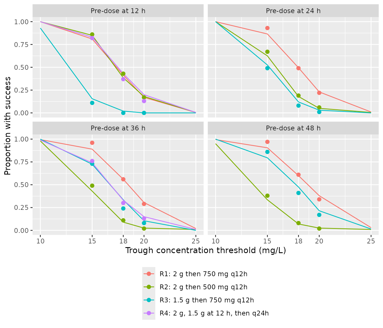
Replicates Figure 2 of Kirwan 2021: proportion of patients whose pre-dose concentration reaches each threshold. Lines = this model (200 virtual patients per regimen); points = digitised Figure 2.
fig2_cmp |>
  dplyr::filter(conc == 15 | conc == 20) |>
  dplyr::mutate(prop_sim = round(prop_sim, 2), diff_pts = round(diff_pts)) |>
  dplyr::select(regimen, time, conc, prop_pub, prop_sim, diff_pts) |>
  dplyr::arrange(regimen, conc, time) |>
  dplyr::rename(
    "Regimen" = regimen, "Time (h)" = time, "Threshold (mg/L)" = conc,
    "Published (Fig. 2)" = prop_pub, "Simulated" = prop_sim,
    "Difference (percentage points)" = diff_pts
  ) |>
knitr::kable(caption = "Probability of a pre-dose level at or above 15 and 20 mg/L.")| Regimen | Time (h) | Threshold (mg/L) | Published (Fig. 2) | Simulated | Difference (percentage points) |
|---|---|---|---|---|---|
| R1: 2 g then 750 mg q12h | 24 | 15 | 0.93 | 0.86 | -7 |
| R1: 2 g then 750 mg q12h | 36 | 15 | 0.96 | 0.89 | -7 |
| R1: 2 g then 750 mg q12h | 48 | 15 | 0.97 | 0.90 | -6 |
| R1: 2 g then 750 mg q12h | 24 | 20 | 0.22 | 0.23 | 1 |
| R1: 2 g then 750 mg q12h | 36 | 20 | 0.29 | 0.30 | 2 |
| R1: 2 g then 750 mg q12h | 48 | 20 | 0.34 | 0.38 | 4 |
| R2: 2 g then 500 mg q12h | 12 | 15 | 0.86 | 0.85 | -1 |
| R2: 2 g then 500 mg q12h | 24 | 15 | 0.67 | 0.62 | -5 |
| R2: 2 g then 500 mg q12h | 36 | 15 | 0.49 | 0.43 | -6 |
| R2: 2 g then 500 mg q12h | 48 | 15 | 0.38 | 0.34 | -4 |
| R2: 2 g then 500 mg q12h | 12 | 20 | 0.17 | 0.18 | 1 |
| R2: 2 g then 500 mg q12h | 24 | 20 | 0.06 | 0.05 | -1 |
| R2: 2 g then 500 mg q12h | 36 | 20 | 0.02 | 0.03 | 1 |
| R2: 2 g then 500 mg q12h | 48 | 20 | 0.02 | 0.03 | 1 |
| R3: 1.5 g then 750 mg q12h | 12 | 15 | 0.11 | 0.16 | 4 |
| R3: 1.5 g then 750 mg q12h | 24 | 15 | 0.49 | 0.52 | 4 |
| R3: 1.5 g then 750 mg q12h | 36 | 15 | 0.73 | 0.72 | -1 |
| R3: 1.5 g then 750 mg q12h | 48 | 15 | 0.86 | 0.80 | -6 |
| R3: 1.5 g then 750 mg q12h | 12 | 20 | 0.00 | 0.00 | 0 |
| R3: 1.5 g then 750 mg q12h | 24 | 20 | 0.01 | 0.03 | 2 |
| R3: 1.5 g then 750 mg q12h | 36 | 20 | 0.08 | 0.10 | 2 |
| R3: 1.5 g then 750 mg q12h | 48 | 20 | 0.17 | 0.22 | 4 |
| R4: 2 g, 1.5 g at 12 h, then q24h | 12 | 15 | 0.82 | 0.83 | 1 |
| R4: 2 g, 1.5 g at 12 h, then q24h | 36 | 15 | 0.76 | 0.74 | -2 |
| R4: 2 g, 1.5 g at 12 h, then q24h | 12 | 20 | 0.13 | 0.20 | 7 |
| R4: 2 g, 1.5 g at 12 h, then q24h | 36 | 20 | 0.13 | 0.15 | 2 |
Agreement is within a few percentage points almost everywhere. The one consistent gap is at the top of regimen 1, where the model reaches 15 mg/L in a few percent fewer patients than the paper (about 0.90 against 0.93-0.97). That is the expected signature of replacing the non-parametric NPAG density with a log-normal of the same CV: the log-normal has a slightly longer lower tail of high-clearance or large-volume patients.
The paper’s Results text reads the same curves in words; for example regimen 3 reaches 15 mg/L in “10-20% at 12 h, 50% at 24 h, 70% at 36 h and > 80% at 48 h”, and “the probability of a level of 25 mg/L was negligible at all investigated time points for each of the simulated dosage regimens”.
p25 <- fig2_sim |> dplyr::filter(conc == 25)
stopifnot(
  # Centre: a mis-transcribed CL, V, dose or infusion rate moves these
  # proportions by tens of percentage points.
  median(abs(fig2_cmp$diff_pts)) < 8,
  # Envelope: robust quantile, not the maximum (each point carries ~3.5
  # percentage points of Monte Carlo error at 200 patients).
  quantile(abs(fig2_cmp$diff_pts), 0.9) < 18,
  # 'Negligible' at 25 mg/L (Results).
  median(p25$prop_sim) < 0.05
)
Which column of Table 3 is the typical value?
Pmetrics reports both the mean and the median of each parameter’s non-parametric distribution, and for this model they differ (CL 2.59 vs 2.70 L/h, V 80.98 vs 73.72 L). The Results text quotes the means. Re-running the same cohort with the medians shows that the means also reproduce the paper’s own PTA simulation more closely, which is why the means are encoded.
mod_median <- mod |> rxode2::ini(lcl = log(2.70), lvc = log(73.72))
#> ℹ change initial estimate of `lcl` to `0.993251773010283`
#> ℹ change initial estimate of `lvc` to `4.30027413280162`
rxode2::rxSetSeed(20211210)
sim_median <- rxode2::rxSolve(mod_median, events = events, keep = "regimen") |>
  as.data.frame()
fig2_median <- dplyr::inner_join(pta_trough(sim_median), fig2_pub,
                                 by = c("regimen_short", "time", "conc")) |>
  dplyr::mutate(diff_pts = 100 * (prop_sim - prop_pub))

tibble::tibble(
  "Typical values" = c("Table 3 means (encoded)", "Table 3 medians"),
  "Median |difference| (points)" = round(c(median(abs(fig2_cmp$diff_pts)),
                                           median(abs(fig2_median$diff_pts))), 1),
  "Mean |difference| (points)" = round(c(mean(abs(fig2_cmp$diff_pts)),
                                         mean(abs(fig2_median$diff_pts))), 1)
) |>
knitr::kable(caption = "Agreement with digitised Figure 2 under each column of Table 3.")| Typical values | Median |difference| (points) | Mean |difference| (points) |
|---|---|---|
| Table 3 means (encoded) | 2 | 3.1 |
| Table 3 medians | 4 | 5.4 |
PKNCA validation: AUC over 24-48 h (Figure S1)
Additional file 1 Figure S1 gives, per regimen, the proportion of simulated patients whose AUC from 24 to 48 h reaches 100-600 mg*h/L. The figure is a vector graphic, so the maintainers read its plotted points exactly from the figure’s drawing coordinates.
sim_nca <- sim |>
  dplyr::filter(!is.na(Cc)) |>
  dplyr::select(id, time, Cc, regimen)

dose_df <- events |>
  dplyr::filter(evid == 1) |>
  dplyr::mutate(duration = amt / rate) |>
  dplyr::select(id, time, amt, duration, regimen)

conc_obj <- PKNCA::PKNCAconc(sim_nca, Cc ~ time | regimen + id)
dose_obj <- PKNCA::PKNCAdose(dose_df, amt ~ time | regimen + id,
                             route = "intravascular", duration = "duration")
intervals <- data.frame(start = 24, end = 48, auclast = TRUE, cmax = TRUE, cmin = TRUE)
nca_res <- PKNCA::pk.nca(PKNCA::PKNCAdata(conc_obj, dose_obj, intervals = intervals))

auc_ind <- as.data.frame(nca_res) |>
  dplyr::filter(PPTESTCD == "auclast") |>
  dplyr::select(id, regimen, auc = PPORRES)
figS1_pub <- tibble::tribble(
  ~regimen_short, ~`100`, ~`200`, ~`300`, ~`400`, ~`500`, ~`600`,
  "R1", 1, 1, 1, 1.000, 0.660, 0.200,
  "R2", 1, 1, 1, 0.628, 0.111, 0.000,
  "R3", 1, 1, 1, 0.935, 0.390, 0.041,
  "R4", 1, 1, 1, 1.000, 0.843, 0.369
) |>
  tidyr::pivot_longer(-regimen_short, names_to = "auc_threshold", values_to = "prop_pub") |>
  dplyr::mutate(auc_threshold = as.numeric(auc_threshold))

figS1_cmp <- auc_ind |>
  dplyr::mutate(regimen_short = substr(regimen, 1, 2)) |>
  tidyr::crossing(auc_threshold = c(100, 200, 300, 400, 500, 600)) |>
  dplyr::group_by(regimen, regimen_short, auc_threshold) |>
  dplyr::summarise(prop_sim = mean(auc >= auc_threshold), .groups = "drop") |>
  dplyr::inner_join(figS1_pub, by = c("regimen_short", "auc_threshold"))

figS1_cmp |>
  dplyr::filter(auc_threshold >= 400) |>
  dplyr::mutate(prop_sim = round(prop_sim, 2)) |>
  dplyr::select(regimen, auc_threshold, prop_pub, prop_sim) |>
  dplyr::rename(
    "Regimen" = regimen, "AUC24-48 threshold (mg*h/L)" = auc_threshold,
    "Published (Fig. S1)" = prop_pub, "Simulated" = prop_sim
  ) |>
knitr::kable(caption = "Probability of AUC24-48 at or above each threshold (all regimens reach 1.00 up to 300 mg*h/L in both).")| Regimen | AUC24-48 threshold (mg*h/L) | Published (Fig. S1) | Simulated |
|---|---|---|---|
| R1: 2 g then 750 mg q12h | 400 | 1.000 | 0.96 |
| R1: 2 g then 750 mg q12h | 500 | 0.660 | 0.69 |
| R1: 2 g then 750 mg q12h | 600 | 0.200 | 0.22 |
| R2: 2 g then 500 mg q12h | 400 | 0.628 | 0.64 |
| R2: 2 g then 500 mg q12h | 500 | 0.111 | 0.10 |
| R2: 2 g then 500 mg q12h | 600 | 0.000 | 0.01 |
| R3: 1.5 g then 750 mg q12h | 400 | 0.935 | 0.90 |
| R3: 1.5 g then 750 mg q12h | 500 | 0.390 | 0.46 |
| R3: 1.5 g then 750 mg q12h | 600 | 0.041 | 0.10 |
| R4: 2 g, 1.5 g at 12 h, then q24h | 400 | 1.000 | 0.98 |
| R4: 2 g, 1.5 g at 12 h, then q24h | 500 | 0.843 | 0.81 |
| R4: 2 g, 1.5 g at 12 h, then q24h | 600 | 0.369 | 0.42 |
The paper’s headline AUC claim is that regimen 1 gives “approximately a 100% probability of attaining a target AUC of 400 mg/L * h for MIC 1 mg/L”.
Comparison against the published AUC24-48
The paper reports no NCA table. The median AUC24-48 of each regimen’s simulated population is, however, fixed by Figure S1: it is the AUC at which the published curve crosses 0.5, obtained here by log-linear interpolation between the two bracketing plotted points.
auc_median_pub <- figS1_pub |>
  dplyr::group_by(regimen_short) |>
  dplyr::arrange(auc_threshold, .by_group = TRUE) |>
  dplyr::summarise(
    auclast = {
      i <- max(which(prop_pub >= 0.5))
      x0 <- auc_threshold[i]; x1 <- auc_threshold[i + 1]
      p0 <- prop_pub[i]; p1 <- prop_pub[i + 1]
      exp(log(x0) + (p0 - 0.5) / (p0 - p1) * log(x1 / x0))
    },
    .groups = "drop"
  ) |>
  dplyr::left_join(dplyr::distinct(auc_ind, regimen) |>
                     dplyr::mutate(regimen_short = substr(regimen, 1, 2)),
                   by = "regimen_short") |>
  dplyr::select(regimen, auclast)

nca_sim_auc <- as.data.frame(nca_res) |>
  dplyr::filter(PPTESTCD == "auclast")

cmp <- nlmixr2lib::ncaComparisonTable(
  simulated = nca_sim_auc,
  reference = auc_median_pub,
  by = "regimen",
  units = c(auclast = "mg*h/L"),
  tolerance_pct = 20
)
knitr::kable(cmp, caption = "Median AUC24-48: simulated vs. read from Figure S1. * differs from reference by >20%.")| NCA parameter | regimen | Reference | Simulated | % diff |
|---|---|---|---|---|
| AUClast (mg*h/L) | R1: 2 g then 750 mg q12h | 533 | 539 | +1.1% |
| AUClast (mg*h/L) | R2: 2 g then 500 mg q12h | 423 | 417 | -1.4% |
| AUClast (mg*h/L) | R3: 1.5 g then 750 mg q12h | 478 | 491 | +2.7% |
| AUClast (mg*h/L) | R4: 2 g, 1.5 g at 12 h, then q24h | 571 | 584 | +2.3% |
auc_pct <- as.data.frame(nca_sim_auc) |>
  dplyr::group_by(regimen) |>
  dplyr::summarise(sim = median(PPORRES), .groups = "drop") |>
  dplyr::inner_join(auc_median_pub, by = "regimen") |>
  dplyr::mutate(pct_diff = 100 * (sim / auclast - 1))
stopifnot(
  # Centre of each regimen's AUC distribution; ~2% Monte Carlo error on a
  # median of 200 patients.
  all(abs(auc_pct$pct_diff) < 10),
  # Regimen 1: 'approximately a 100% probability' of AUC24-48 >= 400.
  mean(auc_ind$auc[startsWith(auc_ind$regimen, "R1")] >= 400) > 0.9
)
Replicate Figure S2 (peak levels after the 36 h dose)
Figure S2 shows the proportion of patients whose concentration after the 36 h dose reaches 20-60 mg/L, read at 38 h for regimens 1-3 and at 39 h for regimen 4 (the 1.5 g dose takes 2.5 h to infuse). As for Figure S1, the plotted points were read exactly from the vector graphic. The paper concludes that none of the regimens carries a risk of peaks above 40 mg/L.
figS2_pub <- tibble::tribble(
  ~regimen_short, ~time, ~conc, ~prop_pub,
  "R1", 38, 20, 0.992, "R1", 38, 30, 0.145, "R1", 38, 40, 0.000,
  "R2", 38, 20, 0.442, "R2", 38, 30, 0.000, "R2", 38, 40, 0.000,
  "R3", 38, 20, 0.928, "R3", 38, 30, 0.035, "R3", 38, 40, 0.000,
  "R4", 39, 20, 1.000, "R4", 39, 30, 0.677, "R4", 39, 40, 0.045
)
figS2_cmp <- sim |>
  dplyr::mutate(regimen_short = substr(regimen, 1, 2)) |>
  dplyr::inner_join(dplyr::distinct(figS2_pub, regimen_short, time),
                    by = c("regimen_short", "time")) |>
  tidyr::crossing(conc = c(20, 30, 40)) |>
  dplyr::group_by(regimen, regimen_short, time, conc) |>
  dplyr::summarise(prop_sim = mean(Cc >= conc), .groups = "drop") |>
  dplyr::inner_join(figS2_pub, by = c("regimen_short", "time", "conc"))

figS2_cmp |>
  dplyr::mutate(prop_sim = round(prop_sim, 2)) |>
  dplyr::select(regimen, time, conc, prop_pub, prop_sim) |>
  dplyr::rename(
    "Regimen" = regimen, "Time (h)" = time, "Threshold (mg/L)" = conc,
    "Published (Fig. S2)" = prop_pub, "Simulated" = prop_sim
  ) |>
knitr::kable(caption = "Probability of a post-dose level at or above each threshold after the 36 h dose.")| Regimen | Time (h) | Threshold (mg/L) | Published (Fig. S2) | Simulated |
|---|---|---|---|---|
| R1: 2 g then 750 mg q12h | 38 | 20 | 0.992 | 0.94 |
| R1: 2 g then 750 mg q12h | 38 | 30 | 0.145 | 0.16 |
| R1: 2 g then 750 mg q12h | 38 | 40 | 0.000 | 0.00 |
| R2: 2 g then 500 mg q12h | 38 | 20 | 0.442 | 0.44 |
| R2: 2 g then 500 mg q12h | 38 | 30 | 0.000 | 0.01 |
| R2: 2 g then 500 mg q12h | 38 | 40 | 0.000 | 0.00 |
| R3: 1.5 g then 750 mg q12h | 38 | 20 | 0.928 | 0.92 |
| R3: 1.5 g then 750 mg q12h | 38 | 30 | 0.035 | 0.10 |
| R3: 1.5 g then 750 mg q12h | 38 | 40 | 0.000 | 0.00 |
| R4: 2 g, 1.5 g at 12 h, then q24h | 39 | 20 | 1.000 | 1.00 |
| R4: 2 g, 1.5 g at 12 h, then q24h | 39 | 30 | 0.677 | 0.71 |
| R4: 2 g, 1.5 g at 12 h, then q24h | 39 | 40 | 0.045 | 0.09 |
Assumptions and deviations
- Mean, not median, typical values. Table 3 prints the mean, SD, CV% and median of each parameter’s NPAG distribution. The means are encoded because the Results text quotes them and because they reproduce the paper’s own PTA simulations (Figure 2) more closely than the medians (see above).
-
Log-normal approximation to a non-parametric
distribution. NPAG estimates a discrete joint distribution of
support points, not a parametric omega. The CV% of Table 3 is carried as
a log-normal variance,
omega^2 = log(CV^2 + 1). Any skew or multimodality of the true distribution (visible as the mean-median gap in V) cannot be recovered from the published table, and no CL-V correlation is reported, so the two random effects are independent. -
Residual error not reported. Neither the Pmetrics
assay-error polynomial nor the fitted gamma/lambda term is given in the
paper or in Additional file 1; both residual terms are carried as
fixed(0). Supply your own residual error before using the model to simulate observed TDM levels. The reproduction of Figures 2, S1 and S2 above without residual error indicates that the paper’s PTA simulations were also of error-free concentrations. - Infusion rate in the PTA simulations. The paper does not state the infusion duration used in its simulations; the ICU’s 10 mg/min policy rate (Methods) is assumed. A 1-h infusion instead changes the simulated 38-39 h peaks by a few percentage points and the troughs and AUC24-48 negligibly.
- Clearance is total clearance. No effluent concentrations were measured, so CL lumps residual native and CVVHDF clearance; the model carries no CVVHDF settings (effluent, dialysate or blood flow) and applies only to patients receiving CVVHDF comparable to the study’s (Prismaflex, PAES filter, blood flow 120-220 mL/min).
- Covariate models not packaged. Table 3 also reports models with clearance split by anticoagulation modality (regional citrate: CL 2.73 L/h; non-citrate: 2.54 L/h) or by vasopressor use (with: 2.73 L/h; without: 2.53 L/h), and example continuous-covariate models (effluent flow, linear; flux, exponential; Additional file 1 Table S1 gives their equation forms). The authors did not select any of them, citing no practical difference from the base model, parameter correlations above 0.9 in the continuous-covariate models, and no gain in the other model-comparison metrics (Additional file 1 Table S2); they used the base model for all dosing simulations. Only the base model is packaged.
-
Level counts. The Abstract reports 155 levels and
the Results text 74 peaks plus 96 troughs (170); both are recorded as
printed in the
populationmetadata. - Digitisation. The Figure 2 values were digitised by the maintainers from the published raster image (about +/-0.02); the Figure S1 and S2 values were read exactly from the vector drawing coordinates of Additional file 1.
- No erratum or correction to Kirwan 2021 was found as of 2026-09-30.