Baricitinib (Decker 2024)
Source:vignettes/articles/Decker_2024_baricitinib.Rmd
Decker_2024_baricitinib.RmdModel and source
- Citation: Decker RL, Steven Ernest C II, Radtke DB, Wang R, Araujo J, Keller SY, Zhang X. A population pharmacokinetic model using allometric scaling for baricitinib in patients with juvenile idiopathic arthritis. CPT Pharmacometrics Syst Pharmacol 2024;13(6):970-981. doi:10.1002/psp4.13131.
- Description: Two-compartment population PK model with zero-order absorption, an absorption lag, and fixed allometric scaling for oral baricitinib in 217 pediatric patients aged 2 to <18 years with polyarticular-course juvenile idiopathic arthritis (JUVE-BASIS, NCT03773978). Apparent total clearance is partitioned semi-mechanistically into an eGFR-dependent apparent renal arm (CLr/F) and an eGFR-independent apparent non-renal arm (CLnr/F). Baseline body weight enters through allometric exponents fixed at 0.75 on all clearance terms (CLr/F, CLnr/F, Q) and at 1 on both volumes (V1/F, V2/F), referenced to 74 kg. The structure was carried unchanged from the adult rheumatoid-arthritis baricitinib population PK model; no further covariate met the stepwise-covariate-modeling inclusion criteria, so the base model is the final model.
- Article: https://doi.org/10.1002/psp4.13131
Baricitinib is an oral Janus-kinase inhibitor. Decker and colleagues took the population PK model previously developed in adult patients with rheumatoid arthritis (RA), added allometric scaling on body weight with the exponents fixed at the canonical 0.75 and 1, and re-estimated it against data from the phase 3 JUVE-BASIS trial in pediatric patients with polyarticular-course juvenile idiopathic arthritis (JIA). The purpose of the analysis was to convert the trial’s age-based dosing into a weight-based posology reproducing the adult 4 mg once-daily exposure. The resulting recommendation - 2 mg once daily for 10 to <30 kg and 4 mg once daily for at least 30 kg - is the approved JIA posology in the European Union.
The structural model is a two-compartment model with zero-order
absorption over a duration D1 after a lag LAG,
dosed directly into the central compartment. Apparent total clearance is
partitioned semi-mechanistically:
-
CLr/F, an apparent renal arm scaled by the patient’s baseline estimated glomerular filtration rate (eGFR, bedside Schwartz), representing renal filtration and secretion - the primary elimination route for baricitinib; -
CLnr/F, an apparent eGFR-independent arm, largely hepatic metabolism.
Body weight enters both arms and Q with an exponent
fixed at 0.75, and both volumes with an exponent fixed at 1, referenced
to 74 kg. No further covariate met the stepwise-covariate-modeling
inclusion criteria, so the base model is the final model.
Population
The analysis dataset contained 1261 baricitinib plasma concentrations from 217 patients aged 2 to <18 years with polyarticular-course JIA (polyarticular RF-positive or RF-negative, extended oligoarticular, enthesitis-related arthritis, or juvenile psoriatic arthritis), all with an inadequate response or intolerance to at least one prior conventional synthetic or biologic DMARD (Table 1). Mean age was 13.3 years (range 2-17) and 79% of patients were in the 12 to <18 year band. Mean body weight was 50.2 kg (range 11.0-111 kg), with 87% of patients weighing at least 30 kg. 150 of 217 patients (69%) were female and 149 (69%) were White; 48 (22%) were Asian. Mean baseline eGFR, computed with the bedside Schwartz equation, was 119 mL/min/1.73 m^2 (range 66.5-201).
Dosing during the trial was age-based: 4 mg once daily for ages 9 to <18 years and 2 mg once daily for ages 2 to <9 years. Of the 1377 concentrations collected, 116 (8%) were excluded, chiefly 106 samples below the 0.200 ng/mL limit of quantification. Safety/PK-period samples were collected as dried whole blood on a Mitra VAMS microsampling device and converted to plasma equivalents using a study-specific blood/plasma ratio of 1.29 (Figure S2), then pooled with the open-label lead-in plasma samples.
The same information is available programmatically via
readModelDb("Decker_2024_baricitinib")()$population.
Source trace
Every ini() entry in
inst/modeldb/specificDrugs/Decker_2024_baricitinib.R
carries an in-file comment naming its origin. They are collected here
for review. All values come from Table 2
(“Pharmacokinetic and covariate parameters in final population PK
model”), Population mean (%SEE) column, unless noted.
| Equation / parameter | Value | Source location |
|---|---|---|
ld1 (D1) |
0.457 h | Table 2, D1 (%SEE 2.76) |
boxcox_d1 |
0.501 | Table 2, “Box-Cox transformation parameter for D1” (%SEE 1.40) |
ltlag (LAG) |
0.147 h | Table 2, LAG (%SEE 2.64) |
lcl_nonren (CLnr/F) |
3.36 L/h | Table 2, CLnr/F (%SEE 4.76) |
lcl_renal (CLr/F) |
6.34 L/h | Table 2, CLr/F (%SEE 2.49) |
lvc (V1/F) |
92.6 L | Table 2, V1/F (%SEE 1.89) |
lq (Q) |
2.67 L/h | Table 2, Q (%SEE 7.64) |
lvp (V2/F) |
25.6 L | Table 2, V2/F (%SEE 12.1) |
e_wt_cl_q |
0.75 (fixed) | Table 2, “Allometric Scaling CL” = 0.75 (FIX); footnotes b, d |
e_wt_vc_vp |
1 (fixed) | Table 2, “Allometric Scaling V” = 1 (FIX); footnotes c, e |
e_dcrcl_cl_renal |
0.00586 | Table 2, “Covariate for change in eGFR on CLr/F” (%SEE 29.0) |
etalcl_nonren variance |
0.539830 | Table 2 BSV 84.6% CV, via footnote a |
etalcl_renal variance |
0.144987 | Table 2 BSV 39.5% CV, via footnote a |
etalvc variance |
0.108176 | Table 2 BSV 33.8% CV, via footnote a |
etalvp variance |
0.277044 | Table 2 BSV 56.5% CV, via footnote a |
etald1 variance |
1.070026 | Table 2 BSV 138.4% CV, via footnote a |
etalq variance |
0.022545 (fixed) | Table 2 BSV 15.1% CV (FIX), via footnote a |
| cov(CLnr/F, CLr/F) | 0.272 | Table 2, “Covariance for CLnr/F and CLr/F”; footnote g |
| cov(CLr/F, V1/F) | -0.00706 | Table 2, “Covariance for CLr and V1/F”; footnote g |
| cov(CLnr/F, V1/F) | 0 (fixed) | Not reported in Table 2; fixed to zero |
propSd |
0.361 | Table 2, “Proportional error”; footnote h: standard deviation |
Total clearance cl <- cl_renal + cl_nonren
|
n/a | Table 2 footnote b |
Allometric scaling (WT/74)^0.75 on CLr/F, CLnr/F,
Q |
n/a | Table 2 footnotes b, d |
Allometric scaling (WT/74)^1.00 on V1/F, V2/F |
n/a | Table 2 footnotes c, e |
Renal-arm eGFR scaling
(CRCL_BASE/93) + 0.00586*(CRCL - CRCL_BASE)
|
n/a | Table 2 footnote f |
Two-compartment structure; zero-order input into
central with duration D1 and lag LAG; no depot state |
n/a | Methods, “Pharmacokinetic model development”; Figure S1 legend (compartments C and Cp only) |
Two conversions are applied when transcribing Table 2.
-
BSV. Footnote a defines the tabulated quantity as
%CV = (sqrt(exp(OMEGA)-1))*100, so the internal variance isOMEGA = log((%CV/100)^2 + 1). Footnote g states that the two covariance entries are already on theomega^2scale, so they are transcribed as-is. -
Concentration units. Doses are in mg and volumes in
L, so
central/vcis in mg/L; the model multiplies by 1000 to reportCcin ng/mL, matching the paper’s exposure units.
Two anchors confirm the transcription independently of any
simulation. At the reference weight of 74 kg and the reference eGFR of
93 mL/min/1.73 m^2 the model gives
CLr/F + CLnr/F = 6.34 + 3.36 = 9.70 L/h, matching the
paper’s statement that “the total clearance estimate (for a weight of 74
kg) is 9.7 L/h”. The reference eGFR of 93 is therefore load-bearing: it
is the median eGFR of the upstream adult analysis, not a
statistic of this pediatric cohort (whose mean baseline eGFR is
119).
# The reported 3x3 block must be positive definite or rxode2's Cholesky
# sampler cannot draw from it. Verify explicitly rather than assume.
om_block <- matrix(
  c(0.539830,  0.272,     0,
    0.272,     0.144987, -0.00706,
    0,        -0.00706,   0.108176),
  nrow = 3, byrow = TRUE,
  dimnames = list(c("CLnr", "CLr", "V1"), c("CLnr", "CLr", "V1"))
)
round(eigen(om_block)$values, 6)
#> [1] 0.678521 0.108545 0.005927
stopifnot(all(eigen(om_block)$values > 0))

# Implied correlations. The CLnr/F - CLr/F pair is very strong but below 1.
round(stats::cov2cor(om_block), 3)
#>       CLnr    CLr     V1
#> CLnr 1.000  0.972  0.000
#> CLr  0.972  1.000 -0.056
#> V1   0.000 -0.056  1.000
Choosing valid validation targets from Table 3
Table 3 reports post-hoc parameter and exposure estimates by age
group and by weight group. Before comparing simulations against it, it
is worth checking which columns are internally consistent: at steady
state under linear PK, AUC(tau,ss) must equal
Dose / (CL/F).
t3 <- tibble::tribble(
  ~group,                  ~dose_mg, ~cl,   ~auc, ~cmax, ~n,
  "2 to <6 y",                    2,  4.87,  410,  87.4,   6,
  "6 to <9 y",                    2,  6.53,  254,  56.8,  10,
  "9 to <12 y",                   4,  8.11,  500,  79.0,  29,
  "12 to <18 y",                  4, 10.30,  386,  57.7, 172,
  "< 30 kg",                      2,  6.30,  464,  85.7,  29,
  ">= 30 kg",                     4, 10.20,  388,  58.1, 188,
  "Adult RA (reference)",         4,  9.42,  483,  53.3, 2393
) |>
  mutate(
    `AUC implied by Dose/CL` = dose_mg / cl * 1000,
    `% difference`           = 100 * (auc - `AUC implied by Dose/CL`) /
                                 `AUC implied by Dose/CL`
  )

t3 |>
  dplyr::rename(
    "Group"                   = group,
    "N"                       = n,
    "Dose (mg)"               = dose_mg,
    "CL/F (L/h)"              = cl,
    "AUCtau,ss reported"      = auc,
    "Cmax,ss reported"        = cmax
  ) |>
  knitr::kable(
    digits  = 1,
    caption = paste(
      "Internal consistency of Decker 2024 Table 3. Under linear steady-state",
      "PK, AUC(tau,ss) must equal Dose/(CL/F)."
    )
)| Group | Dose (mg) | CL/F (L/h) | AUCtau,ss reported | Cmax,ss reported | N | AUC implied by Dose/CL | % difference |
|---|---|---|---|---|---|---|---|
| 2 to <6 y | 2 | 4.9 | 410 | 87.4 | 6 | 410.7 | -0.2 |
| 6 to <9 y | 2 | 6.5 | 254 | 56.8 | 10 | 306.3 | -17.1 |
| 9 to <12 y | 4 | 8.1 | 500 | 79.0 | 29 | 493.2 | 1.4 |
| 12 to <18 y | 4 | 10.3 | 386 | 57.7 | 172 | 388.3 | -0.6 |
| < 30 kg | 2 | 6.3 | 464 | 85.7 | 29 | 317.5 | 46.2 |
| >= 30 kg | 4 | 10.2 | 388 | 58.1 | 188 | 392.2 | -1.1 |
| Adult RA (reference) | 4 | 9.4 | 483 | 53.3 | 2393 | 424.6 | 13.7 |
Four columns reconcile to within about 1.5% (2 to <6 y, 9 to <12 y, 12 to <18 y, and >= 30 kg). Three do not, and each has an identifiable reason:
-
< 30 kgis off by +46%. Its own CL/F of 6.30 L/h with the printed 2 mg dose implies an AUC of 317 ng*h/mL, not the reported 464. The trial dosed by age, not weight, so patients aged 9 years and older who happened to weigh under 30 kg received 4 mg. Back-solving,464 * 6.30 / 1000 = 2.92 mgis the effective mean dose in that column - consistent with roughly 45% of the 29 patients receiving 4 mg. This column is therefore not a valid target for a 2 mg simulation, even though the “Dose (mg)” row prints 2. It is excluded from the comparison below. -
6 to <9 yis off by -17%. Table 3 footnote d records that 2 of the 10 patients received incorrect dosing and were excluded from the dose-dependent parameters, so its AUC and Cmax come from N = 8 while its CL/F comes from N = 10. - Adult RA is off by +14%. Table 3 footnote f states those values are based on all patients in the adult dataset with the dose normalised to 4 mg QD, a different aggregation from the pediatric columns.
The simulations below therefore target the four age groups as
actually dosed in the trial, plus the >= 30 kg weight
group, and flag the two small age groups (N = 6 and N = 8) as
low-precision references rather than firm targets.
Virtual cohort
Original individual data are not publicly available. Each arm below reproduces one Table 3 column, with body weight and baseline eGFR drawn to match the mean and range reported for that group in Table 1, and the dose that group actually received in the trial.
| Arm | Table 1 N | Dose | Weight, mean (range) | Baseline eGFR, mean (range) |
|---|---|---|---|---|
| 2 to <6 y | 6 | 2 mg QD | 14.5 kg (11.0-19.2) | 122 (108-144) |
| 6 to <9 y | 9 | 2 mg QD | 19.7 kg (13.3-26.1) | 141 (102-175) |
| 9 to <12 y | 30 | 4 mg QD | 35.3 kg (21.9-63.5) | 129 (82-179) |
| 12 to <18 y | 172 | 4 mg QD | 55.6 kg (26.1-111) | 116 (66.5-201) |
| >= 30 kg | 188 | 4 mg QD | 54.5 kg (30.3-111) | ~117 (66.5-201) |
The >= 30 kg mean baseline eGFR is not printed in
Table 1 (the cell is blank in the published table); it is recovered from
the paper’s own numbers by mass balance,
(119*217 - 134*29)/188 = 116.7, rounded to 117. The eGFR
range for that stratum is taken as the all-patients range.
set.seed(20240604)

# Rejection-sample a truncated normal matched to a reported mean and range.
rtrunc_norm <- function(n, mean, lo, hi) {
  if (isTRUE(all.equal(lo, hi))) return(rep(mean, n))
  sd  <- (hi - lo) / 4
  out <- numeric(0)
  while (length(out) < n) {
    x   <- stats::rnorm(4 * n, mean = mean, sd = sd)
    out <- c(out, x[x >= lo & x <= hi])
  }
  out[seq_len(n)]
}

# Steady-state design: QD dosing for 7 days, then a densely sampled final
# dosing interval (144-168 h). Terminal t1/2 is ~8 h, so 7 days is > 20
# half-lives and accumulation is complete.
tau      <- 24
n_doses  <- 7L
ss_start <- (n_doses - 1L) * tau          # 144 h -- time of the final dose
obs_grid <- sort(unique(c(
  seq(ss_start,       ss_start + 2,   by = 0.10),   # capture the sharp peak
  seq(ss_start + 2.5, ss_start + 12,  by = 0.50),
  seq(ss_start + 13,  ss_start + tau, by = 1.00)
)))

# Build one arm. `id_offset` keeps IDs disjoint across bind_rows()-ed arms;
# duplicate IDs are silently merged by rxSolve into a single wrong subject.
make_arm <- function(n, amt_mg, wt_mean, wt_lo, wt_hi,
                     egfr_mean, egfr_lo, egfr_hi, treatment, id_offset = 0L) {
  subj <- tibble(
    id        = id_offset + seq_len(n),
    WT        = rtrunc_norm(n, wt_mean, wt_lo, wt_hi),
    CRCL_BASE = rtrunc_norm(n, egfr_mean, egfr_lo, egfr_hi),
    treatment = treatment
  ) |>
    # The paper reports no on-treatment eGFR trajectory, so the time-varying
    # arm is switched off by setting CRCL == CRCL_BASE (delta-eGFR = 0).
    mutate(CRCL = CRCL_BASE)

  doses <- subj |>
    tidyr::crossing(time = seq(0, by = tau, length.out = n_doses)) |>
    mutate(
      amt  = amt_mg,
      evid = 1L,
      cmt  = "central",
      # rate = -2 tells rxode2 the infusion DURATION is modeled -- here by
      # dur(central) <- d1 in the model file. Without it the zero-order
      # absorption duration D1 is ignored and the dose becomes a bolus.
      rate = -2
    )

  obs <- subj |>
    tidyr::crossing(time = obs_grid) |>
    mutate(
      amt  = NA_real_,
      evid = 0L,
      # The ODE state name, never the observable name "Cc" -- referencing an
      # algebraic observable as a compartment renumbers the ODE slots.
      cmt  = "central",
      rate = NA_real_
    )

  bind_rows(doses, obs) |> arrange(id, time, desc(evid))
}

arms <- tibble::tribble(
  ~treatment,     ~amt_mg, ~wt_mean, ~wt_lo, ~wt_hi, ~egfr_mean, ~egfr_lo, ~egfr_hi,
  "2 to <6 y",          2,     14.5,   11.0,   19.2,        122,    108.0,      144,
  "6 to <9 y",          2,     19.7,   13.3,   26.1,        141,    102.0,      175,
  "9 to <12 y",         4,     35.3,   21.9,   63.5,        129,     82.0,      179,
  "12 to <18 y",        4,     55.6,   26.1,  111.0,        116,     66.5,      201,
  ">= 30 kg",           4,     54.5,   30.3,  111.0,        117,     66.5,      201
) |>
  mutate(id_offset = 1000L * seq_len(dplyr::n()))

n_per_arm <- 200L

events <- do.call(bind_rows, lapply(seq_len(nrow(arms)), function(i) {
  a <- arms[i, ]
  make_arm(n_per_arm, a$amt_mg, a$wt_mean, a$wt_lo, a$wt_hi,
           a$egfr_mean, a$egfr_lo, a$egfr_hi, a$treatment, a$id_offset)
}))

stopifnot(!anyDuplicated(unique(events[, c("id", "time", "evid")])))
c(arms = nrow(arms), subjects = dplyr::n_distinct(events$id), rows = nrow(events))
#>     arms subjects     rows
#>        5     1000    60000
Simulation
mod <- readModelDb("Decker_2024_baricitinib")

sim <- rxode2::rxSolve(
  mod,
  events = events,
  keep   = c("treatment", "WT", "CRCL_BASE")
) |>
  as.data.frame()
#> ℹ parameter labels from comments will be replaced by 'label()'

# rxSolve can silently drop subjects; assert the count survived.
stopifnot(dplyr::n_distinct(sim$id) == dplyr::n_distinct(events$id))
c(subjects_out = dplyr::n_distinct(sim$id), rows_out = nrow(sim))
#> subjects_out     rows_out
#>         1000        53000
Structural check against Table 3
Because the model’s only structural covariates are body weight and baseline eGFR, the typical-value parameters evaluated at each group’s mean weight and mean eGFR can be compared directly against the post-hoc geometric means in Table 3. This is deterministic, so between-subject variability is zeroed.
# zeroRe() removes the random effects. omega = NA is passed explicitly because
# rxSolve() otherwise reuses the omega from the previous solve in the session.
mod_typical <- rxode2::zeroRe(mod)
#> ℹ parameter labels from comments will be replaced by 'label()'

typ_events <- do.call(bind_rows, lapply(seq_len(nrow(arms)), function(i) {
  a <- arms[i, ]
  make_arm(1L, a$amt_mg, a$wt_mean, a$wt_mean, a$wt_mean,
           a$egfr_mean, a$egfr_mean, a$egfr_mean, a$treatment, a$id_offset)
}))

sim_typ <- rxode2::rxSolve(
  mod_typical, events = typ_events, omega = NA,
  keep = c("treatment", "WT", "CRCL_BASE")
) |>
  as.data.frame()
#> Warning: multi-subject simulation without without 'omega'

# Terminal (beta) half-life of a two-compartment model from the micro-constants.
terminal_half_life <- function(cl, vc, q, vp) {
  k10  <- cl / vc
  k12  <- q / vc
  k21  <- q / vp
  a    <- k10 + k12 + k21
  beta <- (a - sqrt(a^2 - 4 * k10 * k21)) / 2
  log(2) / beta
}

typ_tbl <- sim_typ |>
  group_by(treatment) |>
  summarise(
    cl_model   = mean(cl),
    v1_model   = mean(vc),
    v2_model   = mean(vp),
    thalf_model = terminal_half_life(mean(cl), mean(vc), mean(q), mean(vp)),
    .groups = "drop"
  )

published_t3 <- tibble::tribble(
  ~treatment,    ~cl_pub, ~v1_pub, ~v2_pub, ~thalf_pub,
  "2 to <6 y",      4.87,    21.7,    4.85,       6.39,
  "6 to <9 y",      6.53,    32.2,    7.92,       8.10,
  "9 to <12 y",     8.11,    49.3,    12.1,       8.47,
  "12 to <18 y",   10.30,    70.8,    16.9,       8.73,
  ">= 30 kg",      10.20,    69.3,    16.8,       8.75
)

typ_tbl |>
  left_join(published_t3, by = "treatment") |>
  mutate(`CL/F % diff` = 100 * (cl_model - cl_pub) / cl_pub,
         `V1/F % diff` = 100 * (v1_model - v1_pub) / v1_pub) |>
  dplyr::rename(
    "Group"               = treatment,
    "CL/F model (L/h)"    = cl_model,
    "CL/F Table 3 (L/h)"  = cl_pub,
    "V1/F model (L)"      = v1_model,
    "V1/F Table 3 (L)"    = v1_pub,
    "V2/F model (L)"      = v2_model,
    "V2/F Table 3 (L)"    = v2_pub,
    "t1/2 model (h)"      = thalf_model,
    "t1/2 Table 3 (h)"    = thalf_pub
  ) |>
  dplyr::relocate(`CL/F % diff`, .after = `CL/F Table 3 (L/h)`) |>
  dplyr::relocate(`V1/F % diff`, .after = `V1/F Table 3 (L)`) |>
  knitr::kable(
    digits  = 1,
    caption = paste(
      "Typical-value structural parameters versus the post-hoc geometric means",
      "of Decker 2024 Table 3."
    )
)| Group | CL/F model (L/h) | V1/F model (L) | V2/F model (L) | t1/2 model (h) | CL/F Table 3 (L/h) | CL/F % diff | V1/F Table 3 (L) | V1/F % diff | V2/F Table 3 (L) | t1/2 Table 3 (h) |
|---|---|---|---|---|---|---|---|---|---|---|
| 12 to <18 y | 9.1 | 69.6 | 19.2 | 9.5 | 10.3 | -11.7 | 70.8 | -1.7 | 16.9 | 8.7 |
| 2 to <6 y | 3.4 | 18.1 | 5.0 | 6.7 | 4.9 | -29.4 | 21.7 | -16.4 | 4.8 | 6.4 |
| 6 to <9 y | 4.8 | 24.7 | 6.8 | 6.8 | 6.5 | -26.4 | 32.2 | -23.4 | 7.9 | 8.1 |
| 9 to <12 y | 7.0 | 44.2 | 12.2 | 8.2 | 8.1 | -14.0 | 49.3 | -10.4 | 12.1 | 8.5 |
| >= 30 kg | 9.0 | 68.2 | 18.9 | 9.4 | 10.2 | -11.6 | 69.3 | -1.6 | 16.8 | 8.8 |
The volume terms reproduce Table 3 closely, which is expected:
V1/F scales linearly with weight (exponent fixed at 1), so
the typical value at the group mean weight and the geometric mean of the
individual estimates should nearly coincide, and they agree to within a
few percent in the two largest groups.
Clearance shows a systematic pattern: the typical value sits below the post-hoc geometric mean, and the gap widens as body weight falls (roughly -12% at 55 kg, growing to about -29% at 14.5 kg). The paper itself supplies the explanation. Its Discussion reports a sensitivity analysis in which the allometric exponents were estimated instead of fixed, returning 0.48 for clearance-related and 0.70 for volume-related parameters. An exponent shallower than 0.75 means clearance falls less steeply as weight decreases, so the fixed-0.75 model necessarily under-predicts clearance in the smallest patients relative to their individual fits. Substituting the paper’s own estimated exponent closes the gap without changing anything else:
# Diagnostic ONLY -- the packaged model keeps the published fixed exponent of
# 0.75 (Table 2, FIX). This recomputes the typical CL/F under the exponent the
# paper's own sensitivity analysis estimated (0.48, Discussion) to show that the
# exponent choice, not a transcription error, drives the residual pattern.
cl_typical <- function(wt, egfr, exponent) {
  (6.34 * (egfr / 93) + 3.36) * (wt / 74)^exponent
}

arms |>
  transmute(
    Group                      = treatment,
    `Weight (kg)`              = wt_mean,
    `CL/F Table 3 (L/h)`       = published_t3$cl_pub[match(treatment, published_t3$treatment)],
    `CL/F at exponent 0.75`    = cl_typical(wt_mean, egfr_mean, 0.75),
    `CL/F at exponent 0.48`    = cl_typical(wt_mean, egfr_mean, 0.48)
  ) |>
  knitr::kable(
    digits  = 2,
    caption = paste(
      "Diagnostic: the fixed 0.75 exponent (the published final model) versus",
      "the 0.48 exponent from the paper's own estimated-exponent sensitivity",
      "analysis. The packaged model uses 0.75."
    )
)| Group | Weight (kg) | CL/F Table 3 (L/h) | CL/F at exponent 0.75 | CL/F at exponent 0.48 |
|---|---|---|---|---|
| 2 to <6 y | 14.5 | 4.87 | 3.44 | 5.34 |
| 6 to <9 y | 19.7 | 6.53 | 4.81 | 6.87 |
| 9 to <12 y | 35.3 | 8.11 | 6.98 | 8.52 |
| 12 to <18 y | 55.6 | 10.30 | 9.09 | 9.82 |
| >= 30 kg | 54.5 | 10.20 | 9.01 | 9.79 |
Replicate published figures
Figure 2 - steady-state concentration-time profiles
Figure 2 of Decker 2024 overlays observed pediatric concentrations on the model-predicted median and 90% prediction interval for adults receiving 4 mg once daily. Observed data are not available, so the panels below show the simulated pediatric prediction interval for each age group at the dose it actually received in the trial.
sim |>
  mutate(time_after_dose = time - ss_start,
         treatment = factor(treatment, levels = arms$treatment)) |>
  group_by(treatment, time_after_dose) |>
  summarise(
    Q05 = quantile(Cc, 0.05, na.rm = TRUE),
    Q50 = quantile(Cc, 0.50, na.rm = TRUE),
    Q95 = quantile(Cc, 0.95, na.rm = TRUE),
    .groups = "drop"
  ) |>
  ggplot(aes(time_after_dose, Q50)) +
  geom_ribbon(aes(ymin = Q05, ymax = Q95), alpha = 0.25) +
  geom_line(linewidth = 0.8) +
  facet_wrap(~treatment) +
  scale_y_log10() +
  labs(
    x = "Time after dose at steady state (h)",
    y = "Baricitinib plasma concentration (ng/mL)",
    title = "Simulated steady-state profiles by trial age group",
    caption = paste(
      "Median with 90% prediction interval,", n_per_arm,
      "virtual patients per arm. Compare with Figure 2 of Decker 2024."
    )
  )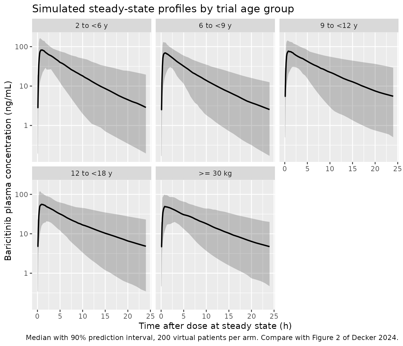
Figure 3 - exposure versus weight band at 1, 2 and 4 mg QD
Figure 3 plots simulated steady-state Cmax and AUC by weight range at 1, 2 and 4 mg once daily against the adult 4 mg reference, and is the analysis that selected the 30 kg cut-off. The paper varied weight in 10 kg steps between 10 and 60 kg and in 20 kg steps between 60 and 120 kg, with eGFR fixed to the study range. The reproduction below uses six weight bands and 100 virtual patients per band-dose arm.
bands <- tibble::tribble(
  ~band,        ~lo,  ~hi,
  "10-20 kg",    10,   20,
  "20-30 kg",    20,   30,
  "30-40 kg",    30,   40,
  "40-60 kg",    40,   60,
  "60-80 kg",    60,   80,
  "80-120 kg",   80,  120
)

grid <- tidyr::crossing(bands, amt_mg = c(1, 2, 4)) |>
  mutate(arm = paste0(band, " | ", amt_mg, " mg"),
         id_offset = 100000L + 1000L * seq_len(dplyr::n()))

events_fig3 <- do.call(bind_rows, lapply(seq_len(nrow(grid)), function(i) {
  g <- grid[i, ]
  make_arm(
    n = 100L, amt_mg = g$amt_mg,
    wt_mean = (g$lo + g$hi) / 2, wt_lo = g$lo, wt_hi = g$hi,
    # eGFR fixed to the study range across all bands, per the paper's Methods.
    egfr_mean = 119, egfr_lo = 66.5, egfr_hi = 201,
    treatment = g$arm, id_offset = g$id_offset
  )
}))

stopifnot(!anyDuplicated(unique(events_fig3[, c("id", "time", "evid")])))
c(arms = nrow(grid), subjects = dplyr::n_distinct(events_fig3$id))
#>     arms subjects
#>       18     1800
sim_fig3 <- rxode2::rxSolve(
  mod, events = events_fig3, keep = c("treatment", "WT")
) |>
  as.data.frame()

stopifnot(dplyr::n_distinct(sim_fig3$id) == dplyr::n_distinct(events_fig3$id))

exposure_fig3 <- sim_fig3 |>
  group_by(treatment, id) |>
  summarise(
    cmax_ss = max(Cc, na.rm = TRUE),
    # Linear-trapezoid AUC over the final dosing interval, for plotting only;
    # the validated NCA comparison below uses PKNCA.
    auc_ss  = sum(diff(time) * (head(Cc, -1) + tail(Cc, -1)) / 2, na.rm = TRUE),
    .groups = "drop"
  ) |>
  tidyr::separate(treatment, into = c("band", "dose_label"), sep = " \\| ",
                  remove = FALSE) |>
  mutate(band = factor(band, levels = bands$band))

# Adult RA reference at 4 mg QD (Decker 2024 Table 3, RA column).
adult_ref <- tibble(metric = c("Cmax,ss (ng/mL)", "AUCtau,ss (ng*h/mL)"),
                    value  = c(53.3, 483))

exposure_fig3 |>
  tidyr::pivot_longer(c(cmax_ss, auc_ss), names_to = "metric") |>
  mutate(metric = ifelse(metric == "cmax_ss",
                         "Cmax,ss (ng/mL)", "AUCtau,ss (ng*h/mL)")) |>
  ggplot(aes(band, value, fill = dose_label)) +
  geom_boxplot(outlier.size = 0.4) +
  geom_hline(data = adult_ref, aes(yintercept = value),
             linetype = "dashed", colour = "red") +
  facet_wrap(~metric, scales = "free_y", ncol = 1) +
  labs(
    x = "Weight band", y = NULL, fill = "Dose",
    title = "Simulated steady-state exposure by weight band and dose",
    caption = paste(
      "Red dashed line: exposure in adult patients with RA at 4 mg QD",
      "(Table 3). Compare with Figure 3 of Decker 2024."
    )
  ) +
  theme(axis.text.x = element_text(angle = 30, hjust = 1))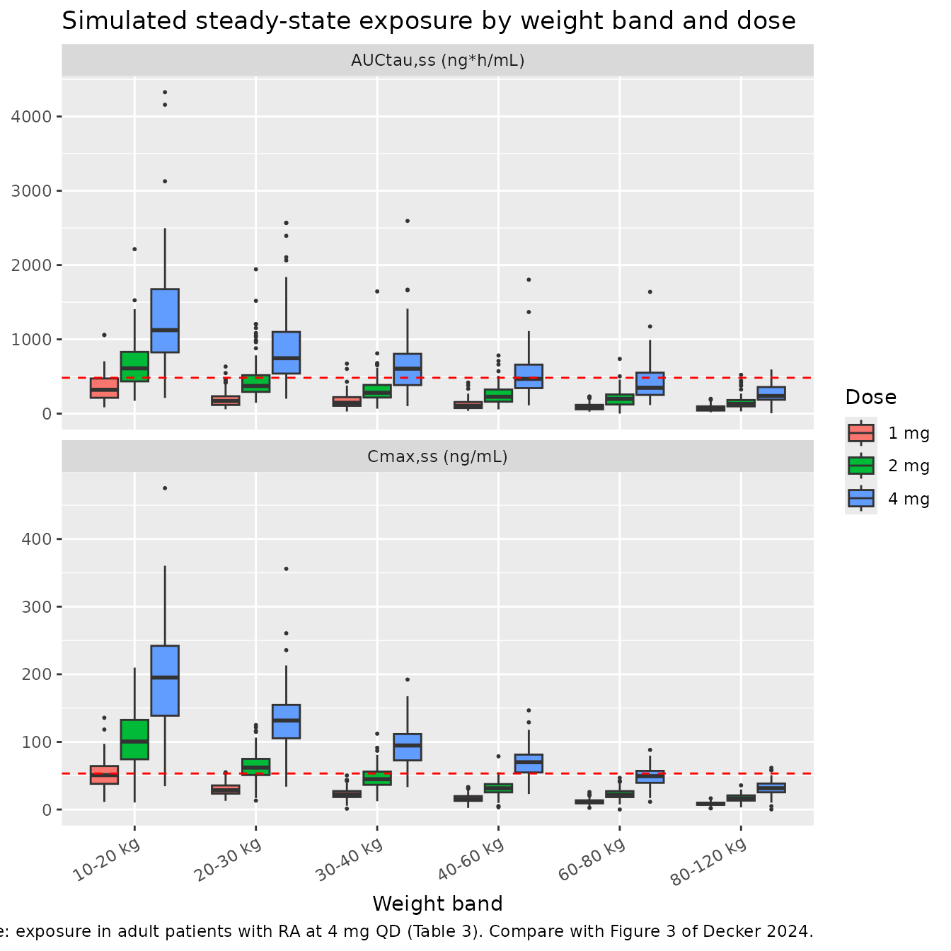
The reproduction supports the paper’s reasoning. At 2 mg QD the 10-20 kg and 20-30 kg bands bracket the adult AUC reference, while 4 mg QD is needed from 30 kg upward; 1 mg QD leaves every band well below the adult AUC, which is why the paper rejected a 1 mg step for the 10-20 kg group despite its closer Cmax match. The paper’s stated reason for preferring AUC matching is that the adult exposure-response analysis found Cmax not to be a relevant driver of efficacy or safety.
PKNCA validation
sim_nca <- sim |>
  filter(!is.na(Cc)) |>
  select(id, time, Cc, treatment)

# Guarantee a record at the interval start (the pre-dose trough at 144 h) so
# PKNCA does not warn about an AUC range starting before the first measurement.
sim_nca <- bind_rows(
  sim_nca,
  sim_nca |> distinct(id, treatment) |> mutate(time = ss_start, Cc = 0)
) |>
  distinct(id, treatment, time, .keep_all = TRUE) |>
  arrange(id, treatment, time)

dose_df <- events |>
  filter(evid == 1) |>
  select(id, time, amt, treatment)

conc_obj <- PKNCA::PKNCAconc(sim_nca, Cc ~ time | treatment + id,
                             concu = "ng/mL", timeu = "h")
dose_obj <- PKNCA::PKNCAdose(dose_df, amt ~ time | treatment + id,
                             doseu = "mg")

# Steady-state interval: the final dosing interval, 144-168 h.
intervals <- data.frame(
  start   = ss_start,
  end     = ss_start + tau,
  cmax    = TRUE,
  tmax    = TRUE,
  cmin    = TRUE,
  auclast = TRUE,
  cav     = TRUE
)

nca_res <- PKNCA::pk.nca(
  PKNCA::PKNCAdata(conc_obj, dose_obj, intervals = intervals)
)
Comparison against published NCA
auclast over the 144-168 h interval is the model’s
AUC(tau,ss) and cmax is Cmax,ss. The
< 30 kg column is excluded for the reason established
above (its reported exposure reflects age-based dosing at an effective
2.92 mg, not the 2 mg printed in its Dose row).
published <- tibble::tribble(
  ~treatment,     ~cmax, ~auclast,
  "2 to <6 y",     87.4,      410,
  "6 to <9 y",     56.8,      254,
  "9 to <12 y",    79.0,      500,
  "12 to <18 y",   57.7,      386,
  ">= 30 kg",      58.1,      388
)

cmp <- nlmixr2lib::ncaComparisonTable(
  simulated     = nca_res,
  reference     = published,
  by            = "treatment",
  units         = c(cmax = "ng/mL", auclast = "ng*h/mL"),
  tolerance_pct = 20
)

knitr::kable(
  cmp,
  caption = paste(
    "Simulated versus published steady-state exposure (Decker 2024 Table 3).",
    "* differs from the reference by more than 20%."
  ),
  align = c("l", "l", "r", "r", "r")
)| NCA parameter | treatment | Reference | Simulated | % diff |
|---|---|---|---|---|
| Cmax (ng/mL) | 2 to <6 y | 87.4 | 94.9 | +8.6% |
| Cmax (ng/mL) | 6 to <9 y | 56.8 | 76.6 | +34.9%* |
| Cmax (ng/mL) | 9 to <12 y | 79 | 86.8 | +9.9% |
| Cmax (ng/mL) | 12 to <18 y | 57.7 | 63.3 | +9.7% |
| Cmax (ng/mL) | >= 30 kg | 58.1 | 57.3 | -1.4% |
| AUClast (ng*h/mL) | 2 to <6 y | 410 | 569 | +38.8%* |
| AUClast (ng*h/mL) | 6 to <9 y | 254 | 432 | +70.1%* |
| AUClast (ng*h/mL) | 9 to <12 y | 500 | 614 | +22.7%* |
| AUClast (ng*h/mL) | 12 to <18 y | 386 | 465 | +20.4%* |
| AUClast (ng*h/mL) | >= 30 kg | 388 | 455 | +17.3% |
- differs from reference by more than ±20%.
Cmax reproduces within about 10% in four of the five
arms (+8.6%, +9.9%, +9.7% and -1.4%), and is closest of all in the
largest arm, >= 30 kg (N = 188, -1.4%). That is the
expected consequence of the volume terms matching: Cmax at steady state
is governed chiefly by V1/F, whose allometric exponent is
fixed at 1 and whose typical values agree with Table 3 to within a few
percent. The one starred Cmax row, 6 to <9 y at +34.9%, is the arm
whose published Cmax comes from only 8 patients after two were excluded
for incorrect dosing (Table 3 footnote d).
AUC is over-predicted throughout: +17.3% for
>= 30 kg and +20.4% for 12 to <18 y - the two large,
well-determined arms - rising to +38.8% and +70.1% in the two smallest
age groups (N = 6 and N = 8). Three effects compound here, none of them
a transcription choice:
-
AUC = Dose / (CL/F), so the clearance under-prediction diagnosed in the structural check reappears as an AUC over-prediction of the same relative size. The driver is the published model’s fixed 0.75 allometric exponent; the paper’s own estimated-exponent analysis returned 0.48, and substituting it closes the gap (see the diagnostic table above). - The simulated summaries are geometric means over a weight
distribution, while the typical-value calculation uses the mean
weight. Because
WT^0.75is concave, the geometric-mean clearance over a spread of weights falls below the clearance at the mean weight, adding a few percent more AUC. The effect is largest in the widest arms. - The two smallest age groups rest on N = 6 and N = 8 post-hoc
geometric means drawn from a population with a between-subject CV of
84.6% on
CLnr/F. Their sampling precision is very low, so they are context rather than targets.
No parameter was adjusted to improve any of these comparisons.
Assumptions and deviations
- Weight and eGFR distributions are reconstructed, not observed. Individual covariates are not published. Each arm’s weight and baseline eGFR are drawn from truncated normals matched to the mean and min/max reported in Table 1. The true distributions are skewed within groups, so the simulated exposure spread will not match the published CV% exactly.
-
The
>= 30 kgmean baseline eGFR is derived, not printed. Table 1 leaves that cell blank in the published table; it is recovered by mass balance from the all-patient mean (119), the< 30 kgmean (134) and the two group sizes (188 and 29), giving 116.7, rounded to 117. -
The
< 30 kgexposure column is not used as a validation target. Its reported AUC and Cmax reflect the trial’s age-based dosing, under which patients aged 9 years and older weighing under 30 kg received 4 mg. Its AUC is inconsistent with its own CL/F at the printed 2 mg dose by +46%, implying an effective dose of 2.92 mg. -
The time-varying eGFR arm is switched off. The
model carries the Wahlby 2004 baseline/difference decomposition of eGFR,
but the paper reports no on-treatment eGFR trajectory and no
distribution for the change from baseline. All simulations here set
CRCL = CRCL_BASE, so the delta term contributes nothing and renal clearance scales only with baseline eGFR. Users with longitudinal eGFR data should populate both columns. -
cov(CLnr/F, V1/F) is fixed to zero. Table 2 reports
covariances for the CLnr/F-CLr/F and CLr/F-V1/F pairs but not for
CLnr/F-V1/F. The unreported element is encoded as
fixed(0)rather than estimated. The resulting 3x3 block is positive definite (verified in the Source trace section; minimum eigenvalue 0.0059). - Simulated AUC runs 17-20% above Table 3 in the well-determined arms. This is a property of the published fixed-exponent model as encoded, not an unresolved transcription question: the structural check localises it to clearance, and the paper’s own estimated-exponent sensitivity analysis (0.48 rather than the fixed 0.75) accounts for it. Nothing was tuned to reduce it.
-
Allometric exponents are the fixed values, not the estimated
ones. The Discussion reports a sensitivity analysis in which
the exponents were estimated rather than fixed, returning 0.48 for
clearance-related and 0.70 for volume-related parameters. Those are
explicitly not the final model - Table 2 reports 0.75 and 1 with
FIX- so only the fixed values are encoded. The 0.48 exponent appears in this vignette solely as a diagnostic explaining the clearance residual, and the paper notes the weight-based dose recommendation is unchanged either way. -
Half-life is computed analytically, not by NCA. The
Table 3
t1/2values derive from post-hoc individual parameters. Estimating a terminal half-life by regression within a single 24 h steady-state interval is biased when the half-life is ~8 h, so the structural comparison uses the analytic two-compartment terminal (beta) half-life andhalf.lifeis omitted from the PKNCA interval specification. - Adult RA values are context, not model content. The adult exposures quoted (AUC(tau,ss) 483 ng*h/mL, Cmax,ss 53.3 ng/mL) come from Table 3 and are used only as a reference line. The adult RA model itself is a separate publication and is not encoded here.
-
No covariate beyond weight and renal function is in the
model. Age, sex, race, ethnicity, Japanese versus non-Japanese,
and JIA subtype were all screened by stepwise covariate modeling and
none met the forward-inclusion criteria (p <= 0.01 and a >= 5%
reduction in the relevant BSV), so backward exclusion was never run and
the base model became the final model. The screened-but-excluded
covariates are recorded in the model file’s
covariatesDataExcludedmetadata. - The blood-to-plasma conversion is upstream of the model. Safety/PK-period whole-blood microsamples were multiplied by 1.29 before modeling; the model operates on plasma-equivalent concentrations only.