Gentamicin (Singu 2024)
Source:vignettes/articles/Singu_2024_gentamicin.Rmd
Singu_2024_gentamicin.RmdModel and source
- Citation: Singu BS, Verbeeck RK, Pieper CH, Ette EI. Confirming the suitability of a gentamicin dosing strategy in neonates using the population pharmacokinetic approach with truncated sampling duration. Children (Basel). 2024;11(8):898. doi:10.3390/children11080898.
- Article: https://doi.org/10.3390/children11080898
- No supplementary material was published; the Data Availability Statement offers the raw data “on request”, so every value below comes from the main article text, tables, and figures.
Population
Singu 2024 is a prospective, non-randomised observational study run in the Neonatal Unit of the Maternity Ward at Windhoek Central Hospital, Namibia. Of 52 enrolled neonates with suspected or confirmed sepsis, 50 were pharmacokinetically evaluable and each contributed exactly two serum samples, for 100 observations in total. Baseline demographics (Table 1) give a median birth weight of 1.57 kg (range 0.90-3.92), median gestational age 32 weeks (24-40) with 43/52 (82.7%) preterm at < 37 weeks, median postnatal age 4.0 days (1.0-17), median white blood cell count 11.0 x 10^9/L (1.67-37.4), and median serum creatinine 0.72 mg/dL (0.20-1.66). 44.2% were female.
Every neonate received gentamicin 5 mg/kg as an intravenous bolus over 3-5 s every 24 h (median dose 7.9 mg, range 4.0-17), combined with benzylpenicillin 100,000 IU/kg q12h or ampicillin 50 mg/kg q8h.
The distinguishing design feature is a truncated sampling duration: samples were confined to the first 7.5 h after a dose, allocated across three informative blocks (8% at 0.08-0.14 h, 68% at 0.14-4.2 h, 24% at 4.2 h and later). This is much shorter than the profiles used by studies that fit two-compartment gentamicin models, and the authors’ thesis is that the block-randomised design still recovers efficient CL and V estimates.
The same information is available programmatically via
readModelDb("Singu_2024_gentamicin")()$population.
Source trace
| Equation / parameter | Value | Source location |
|---|---|---|
| One-compartment linear IV structure | n/a | Results 3.3 (one-compartment OFV 15.076 vs two-compartment 7602.386); Conclusions |
lcl (CL before maturation) |
0.196 L/h | Table 3, “CL (L/h)” |
lvc |
0.417 L | Table 3, “V (L)” |
e_wt_birth_cl |
1.30 | Table 3, “CL_WT” |
e_wt_birth_vc |
1.76 | Table 3, “V_WT” |
e_wbc_cl |
-0.560 | Table 3, “CL_WBC” |
e_pna_cl_hill (GAMMA) |
0.551 (fixed) | Table 3, “GAMMA” (CI column reads “Fixed”); Table 3 footnote |
lpna50 (PNA50) |
0.0332 yr (fixed) | Table 3, “PNA 50 (yr)” (CI column reads “Fixed”); Table 3 footnote |
| CL covariate equation | n/a | Equation 3, page 7 |
| FMAT logistic age function | n/a | Equation 2 (generic form) + Results 3.4 and Table 2 footnote
(PNA^GAMMA / (PNA^GAMMA + PNA50^GAMMA)) |
| V covariate equation | n/a | Equation 4, page 7 |
etalcl / etalvc block |
1.00e-5, 0.00024, 0.501 | Table 3, “omega^2 CL”, “omega^2 CL:V”, “omega^2 V” |
etalpna50 |
6.23 | Table 3, “omega^2 PNA 50” |
propSdLow / addSdLow
|
0.99 / 4.96 ng/mL | Table 3, “Res PROPORTIONAL1” / “Res ADDITIVE1” |
propSdHigh / addSdHigh
|
0.0205 / 1.00e-5 ng/mL | Table 3, “Res PROPORTIONAL2” / “Res ADDITIVE2” |
| Residual-error threshold | 2264.25 ng/mL (quoted as log(concentration) = 7.725) | Results 3.4, final paragraph |
| Typical-value cross-check | CL 0.069 L/h, V 0.417 L, t1/2 4.2 h | Results 3.4 |
| Observed concentration range | log(mg/L) about -2.2 to 4.1 over 0-7 h | Figure 1 |
| Simulated exposure by PNA / birth weight | Cmin and Cmax percentiles | Table 4 (not reproducible; see below) |
mod <- readModelDb("Singu_2024_gentamicin")Structural verification against the paper’s own typical values
The paper states (Results 3.4) that for the typical neonate – birth weight 1.57 kg, postnatal age 4 days (0.011 years), log-transformed WBC 2.39 – the predicted CL and V are 0.069 L/h and 0.417 L, and that the resulting elimination half-life is 4.2 h. Those three numbers are the tightest published check on the whole covariate chain, because reproducing CL requires the birth-weight term, the WBC term, and the maturation function to all be encoded correctly.
omega = NA is used to zero the random effects for this
one solve. rxode2::zeroRe() is deliberately
not used: it mutates the model object, so it would
silently strip the IIV from every later simulation in this vignette.
pna_months_4d <- 4 / 30.4375  # canonical PNA column is in months

ev_typ <- rxode2::et(amt = 5 * 1.57, cmt = "central") |>
  rxode2::et(seq(0, 24, by = 0.05))

sim_typ <- rxode2::rxSolve(
  mod, ev_typ,
  params = c(WT_BIRTH = 1.57, PNA = pna_months_4d, WBC = 11.0),
  omega = NA
) |>
  as.data.frame()
#> ℹ parameter labels from comments will be replaced by 'label()'

# Random effects really are off: with etas at zero, vc must equal the
# covariate-only prediction exactly.
stopifnot(isTRUE(all.equal(unique(sim_typ$vc), 0.417, tolerance = 1e-8)))

typical_check <- tibble::tibble(
  Quantity  = c("CL (L/h)", "V (L)", "Half-life (h)", "FMAT (maturation on CL)"),
  Model     = c(sim_typ$cl[1], sim_typ$vc[1],
                log(2) * sim_typ$vc[1] / sim_typ$cl[1],
                sim_typ$maturation_cl[1]),
  Published = c(0.069, 0.417, 4.2, NA_real_)
)

typical_check |>
  knitr::kable(digits = 4,
caption = "Model reproduction of the typical-neonate values stated in Singu 2024 Results 3.4.")| Quantity | Model | Published |
|---|---|---|
| CL (L/h) | 0.0688 | 0.069 |
| V (L) | 0.4170 | 0.417 |
| Half-life (h) | 4.1995 | 4.200 |
| FMAT (maturation on CL) | 0.3518 | NA |
The FMAT value has no directly published counterpart, but it is
reproducible by hand from the paper’s fixed GAMMA and PNA50:
0.011^0.551 / (0.011^0.551 + 0.0332^0.551) = 0.35236. This
arithmetic also falsifies the competing reading of
Equation 2, in which the denominator would carry a bare
PNA50 rather than PNA50^GAMMA: that form gives
FMAT = 0.7151 and hence CL = 0.14 L/h, which contradicts the paper’s own
0.069 L/h. The exponentiated form used here is the one printed in
Results 3.4 and in the Table 2 footnote.
Covariate relationships
grid_pna <- tibble::tibble(PNA_days = seq(0.25, 30, by = 0.25)) |>
  mutate(
    PNA_yr = PNA_days / 365.25,
    FMAT   = PNA_yr^0.551 / (PNA_yr^0.551 + 0.0332^0.551)
  )

p_mat <- ggplot(grid_pna, aes(PNA_days, FMAT)) +
  geom_line(linewidth = 0.9) +
  geom_vline(xintercept = 0.0332 * 365.25, linetype = "dashed") +
  geom_hline(yintercept = 0.5, linetype = "dotted") +
  labs(x = "Postnatal age (days)", y = "FMAT",
       title = "CL maturation",
       subtitle = "Dashed line: PNA50 = 0.0332 yr = 12.1 days") +
  theme_bw()

grid_wbc <- tibble::tibble(WBC = seq(1.67, 37.4, length.out = 200)) |>
  mutate(factor = (log(WBC) / 2.39)^(-0.560))

p_wbc <- ggplot(grid_wbc, aes(WBC, factor)) +
  geom_line(linewidth = 0.9) +
  geom_hline(yintercept = 1, linetype = "dotted") +
  labs(x = "WBC (10^9/L)", y = "CL multiplier",
       title = "WBC effect on CL",
       subtitle = "Reference log(WBC) = 2.39 (WBC 11.0)") +
  theme_bw()

p_mat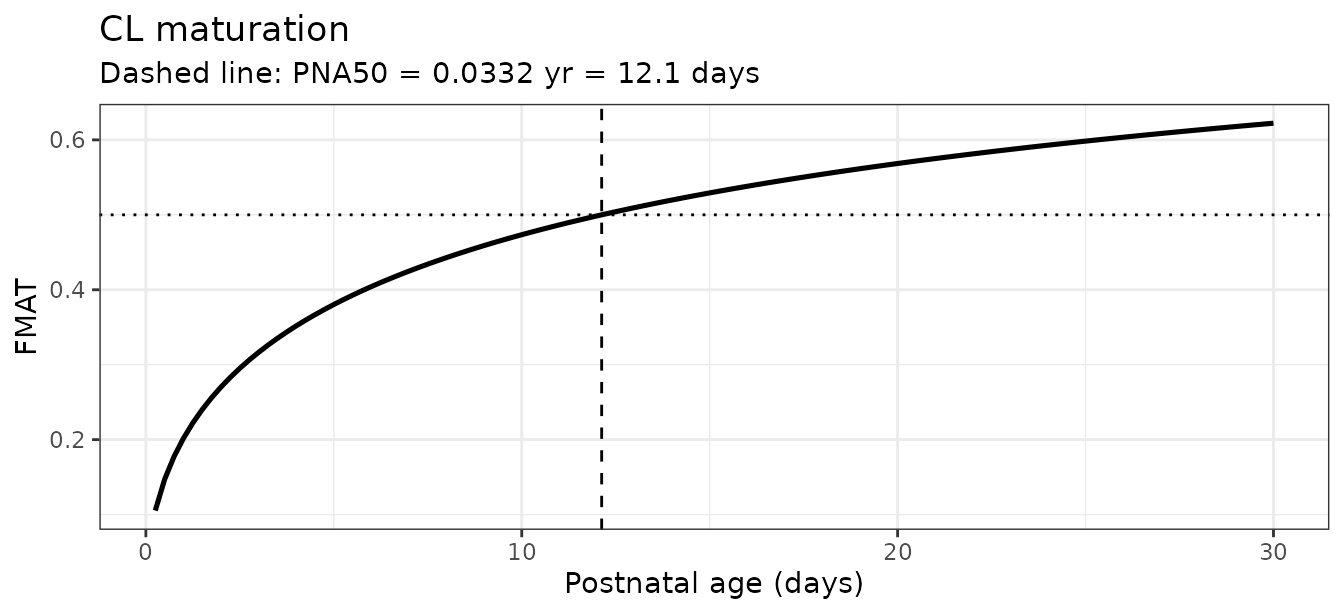
p_wbc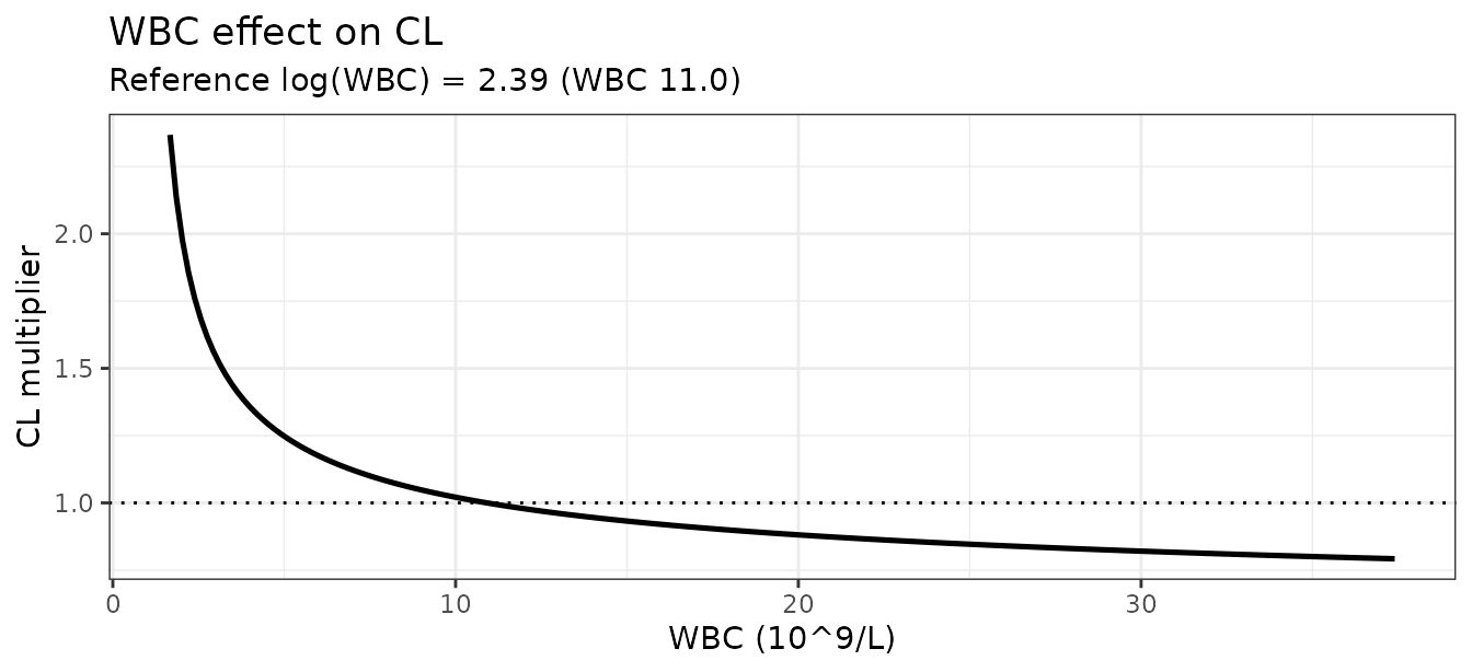
Across the observed WBC range the multiplier spans 0.792 to 2.368, i.e. higher WBC lowers clearance – the direction the Discussion attributes to sepsis-associated inflammation causing acute kidney injury and a fall in eGFR.
Virtual cohort
Original observed data are not publicly available. The cohort below draws covariates from truncated log-normal distributions whose medians and ranges match Table 1.
set.seed(20240726)

rtrunc_lnorm <- function(n, med, lo, hi, sdlog) {
  x <- stats::rlnorm(n, meanlog = log(med), sdlog = sdlog)
  pmin(pmax(x, lo), hi)
}

n_main <- 200L

subjects <- tibble::tibble(
  id       = seq_len(n_main),
  WT_BIRTH = rtrunc_lnorm(n_main, 1.57, 0.90, 3.92, 0.35),
  PNA_days = rtrunc_lnorm(n_main, 4.0, 1.0, 17.0, 0.58),
  WBC      = rtrunc_lnorm(n_main, 11.0, 1.67, 37.4, 0.60)
) |>
  mutate(PNA = PNA_days / 30.4375)

obs_times <- sort(unique(c(seq(0, 7.5, by = 0.25), seq(8, 24, by = 0.5))))

doses <- subjects |>
  transmute(id, time = 0, amt = 5 * WT_BIRTH, evid = 1L,
            cmt = "central", WT_BIRTH, PNA, WBC)

obs <- subjects |>
  tidyr::crossing(time = obs_times) |>
  transmute(id, time, amt = NA_real_, evid = 0L,
            cmt = "central", WT_BIRTH, PNA, WBC)

events <- bind_rows(doses, obs) |> arrange(id, time, desc(evid))

# One dose row and one observation row may share time 0; nothing else may
# repeat an (id, time, evid) triple.
stopifnot(anyDuplicated(events[, c("id", "time", "evid")]) == 0L)
Simulation
rxSolve() returns only the observation rows, so there is
no evid column on the result – evid lives on
the event table that goes in, not on the solve that comes out.
sim <- rxode2::rxSolve(mod, events = events,
                       keep = c("WT_BIRTH", "PNA", "WBC")) |>
  as.data.frame()

# rxSolve silently drops subjects on some failures -- assert the count.
stopifnot(dplyr::n_distinct(sim$id) == n_main)
stopifnot(!"evid" %in% names(sim))

# The IIV really is applied: dividing out the covariate model must leave a
# spread equal to the reported omega on V (sqrt(0.501) = 0.708).
eta_v_recovered <- sim |>
  distinct(id, .keep_all = TRUE) |>
  mutate(eta = log(vc / (0.417 * (WT_BIRTH / 1.57)^1.76))) |>
  pull(eta)
stopifnot(abs(stats::sd(eta_v_recovered) - sqrt(0.501)) < 0.15)
Replicating Figure 1 (log concentration vs time, truncated window)
Figure 1 of Singu 2024 is a scatter/spaghetti plot of
Log (Concentration) against time over the truncated 0-7 h
sampling window. Its y-axis spans about -2.2 to 4.1, with the bulk of
the two-point profiles between roughly 1.5 and 3.5 and a single much
lower profile running from about -0.85 down to -2.15. That axis is
therefore natural-log mg/L (equivalently log ug/mL):
exp(4.1) is 60 mg/L and exp(-2.2) is 0.11
mg/L, both plausible gentamicin serum values, whereas a ng/mL axis would
have put every point between 5.7 and 11.
The panel below draws the same view from the packaged model using the
simulated observations (sim, i.e. including residual
error).
sim |>
  filter(time >= 0.08, time <= 7.5, sim > 0) |>
  ggplot(aes(time, log(sim), group = id)) +
  geom_line(alpha = 0.25, linewidth = 0.3) +
  labs(x = "Time (h)", y = "Log (Concentration in mg/L)",
       title = "Figure 1 - gentamicin concentration-time profiles",
       caption = "Replicates Figure 1 of Singu 2024 (truncated 7.5 h window).") +
  theme_bw()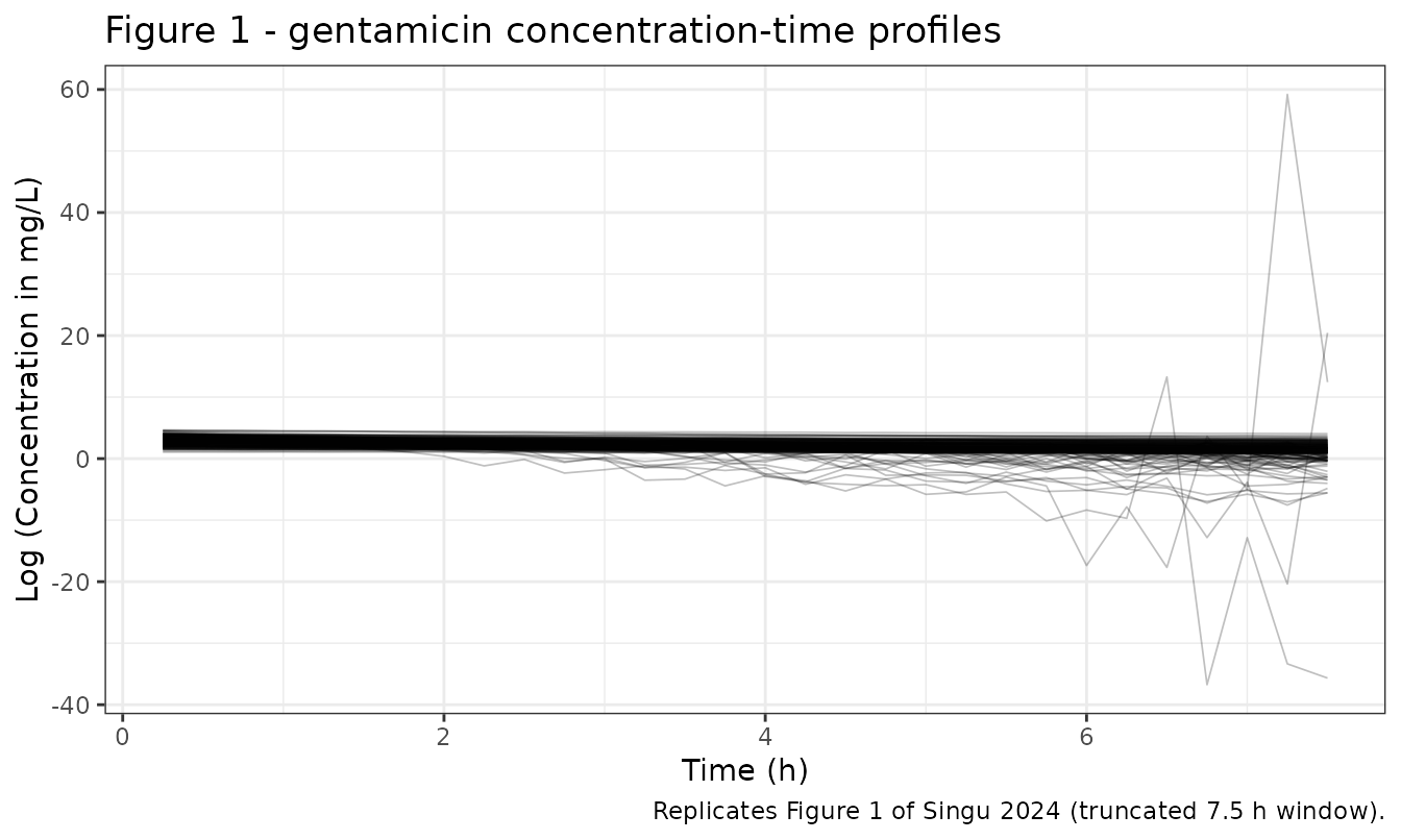
Figure 1 also settles which of the two residual-error tiers is the
data-rich one. The residual threshold is 2264.25 ng/mL,
i.e. 2.264 mg/L, which on Figure 1’s axis is
log(2.264) = 0.817. Almost every plotted observation sits
above that line; only the one low profile (and the tail of one other)
falls below it. The high-concentration stratum therefore carries
essentially all 100 observations, and the sparse low tail is the stratum
whose residual SD is large and poorly determined. That is the basis for
the tier assignment discussed under Assumptions and
deviations.
Concentration-time percentiles over one dosing interval
sim |>
  group_by(time) |>
  summarise(Q05 = quantile(Cc, 0.05), Q50 = quantile(Cc, 0.50),
            Q95 = quantile(Cc, 0.95), .groups = "drop") |>
  ggplot(aes(time, Q50)) +
  geom_ribbon(aes(ymin = Q05, ymax = Q95), alpha = 0.25) +
  geom_line(linewidth = 0.8) +
  geom_hline(yintercept = c(2, 5, 12), linetype = "dashed", colour = "grey40") +
  scale_y_log10() +
  labs(x = "Time (h)", y = "Gentamicin (mg/L)",
       title = "Simulated 5 mg/kg q24h profile, median with 5th-95th percentiles",
       caption = paste("Dashed lines: trough target < 2 mg/L and peak target",
                       "5-12 mg/L (Introduction).")) +
  theme_bw()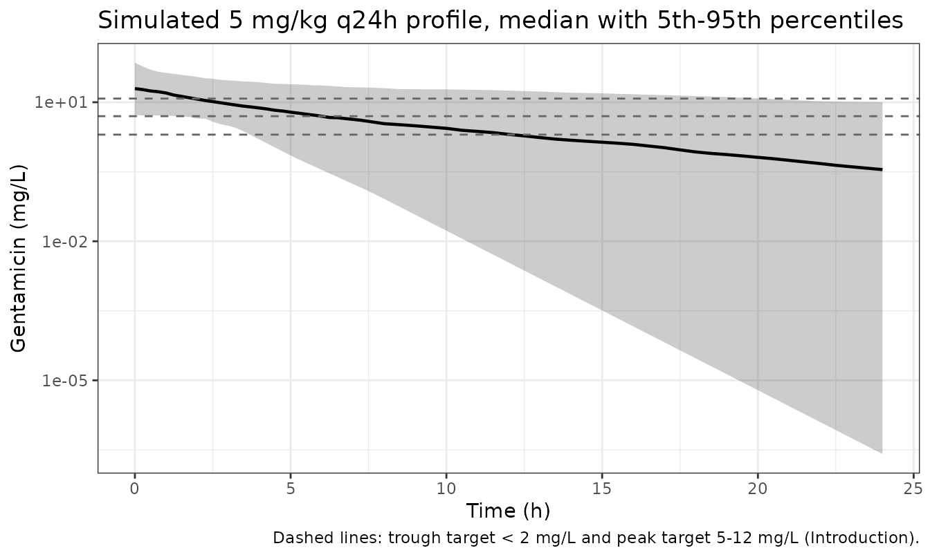
PKNCA validation
NCA is run on the noise-free individual predictions
(Cc), for the typical neonate and for the virtual cohort as
two treatment groups.
sim_typ_nca <- sim_typ |>
  transmute(id = 1L, time, Cc, treatment = "Typical neonate")

sim_pop_nca <- sim |>
  filter(!is.na(Cc)) |>
  transmute(id = id + 1000L, time, Cc, treatment = "Virtual cohort")

sim_nca <- bind_rows(sim_typ_nca, sim_pop_nca) |>
  distinct(treatment, id, time, .keep_all = TRUE) |>
  arrange(treatment, id, time)

# IV bolus: the t = 0 record is the post-dose peak, not a zero. Assert that
# every subject has one rather than inserting a Cc = 0 row (which would be
# correct only for extravascular dosing).
stopifnot(all(
  sim_nca |> group_by(treatment, id) |> summarise(has0 = any(time == 0),
                                                  .groups = "drop") |> pull(has0)
))

dose_df <- bind_rows(
  tibble::tibble(id = 1L, time = 0, amt = 5 * 1.57,
                 treatment = "Typical neonate"),
  doses |> transmute(id = id + 1000L, time, amt, treatment = "Virtual cohort")
)

conc_obj <- PKNCA::PKNCAconc(sim_nca, Cc ~ time | treatment + id)
dose_obj <- PKNCA::PKNCAdose(dose_df, amt ~ time | treatment + id)

intervals <- data.frame(
  start = 0, end = Inf,
  cmax = TRUE, tmax = TRUE, aucinf.obs = TRUE,
  half.life = TRUE, cl.obs = TRUE, vz.obs = TRUE
)

nca_res <- PKNCA::pk.nca(PKNCA::PKNCAdata(conc_obj, dose_obj,
                                          intervals = intervals))

nca_res$result |>
  filter(start == 0, end == Inf) |>
  group_by(treatment, PPTESTCD) |>
  summarise(Median = stats::median(PPORRES), .groups = "drop") |>
  tidyr::pivot_wider(names_from = treatment, values_from = Median) |>
  mutate(PPTESTCD = nlmixr2lib::ncaParamLabel(PPTESTCD)) |>
  dplyr::rename("NCA parameter" = PPTESTCD) |>
  knitr::kable(digits = 3,
               caption = "Median PKNCA results by group (noise-free Cc input).")
#> Warning: There was 1 warning in `mutate()`.
#> ℹ In argument: `PPTESTCD = nlmixr2lib::ncaParamLabel(PPTESTCD)`.
#> Caused by warning:
#> ! ncaParamLabel(): unknown PKNCA code(s) returned as-is: 'adj.r.squared', 'clast.pred', 'lambda.z.time.first', 'lambda.z.time.last', 'r.squared', 'span.ratio'| NCA parameter | Typical neonate | Virtual cohort |
|---|---|---|
| adj.r.squared | 1.000 | 1.000 |
| AUC0-∞ (obs) | 114.054 | 118.881 |
| CL/F | 0.069 | 0.067 |
| Clast | 0.358 | 0.352 |
| clast.pred | 0.358 | 0.352 |
| Cmax | 18.825 | 19.707 |
| t½ | 4.200 | 4.287 |
| λz | 0.165 | 0.162 |
| λz n points | 480.000 | 63.000 |
| lambda.z.time.first | 0.050 | 0.250 |
| lambda.z.time.last | 24.000 | 24.000 |
| r.squared | 1.000 | 1.000 |
| span.ratio | 5.703 | 5.540 |
| Tlast | 24.000 | 24.000 |
| Tmax | 0.000 | 0.000 |
| Vz/F | 0.417 | 0.428 |
Comparison against published values
The paper reports no NCA table. The three quantities it does publish
for the typical neonate – CL, V, and half-life – are the reference set;
for a one-compartment bolus with noise-free input, cl.obs
and vz.obs must recover the model’s CL and V exactly, so
this is a closed-form check of the whole covariate chain rather than a
soft comparison.
published <- tibble::tribble(
  ~treatment,        ~cl.obs, ~vz.obs, ~half.life,
  "Typical neonate", 0.069,   0.417,   4.2
)

simulated_typ <- nca_res$result |>
  filter(treatment == "Typical neonate", start == 0, end == Inf)

cmp <- nlmixr2lib::ncaComparisonTable(
  simulated = simulated_typ,
  reference = published,
  by        = "treatment",
  units     = c(cl.obs = "L/h", vz.obs = "L", half.life = "h"),
  tolerance_pct = 20
)

knitr::kable(
  cmp,
  caption = paste("Simulated vs published NCA for the typical neonate,",
                  "Singu 2024 Results 3.4.",
                  "* differs from reference by >20%.")
)| NCA parameter | treatment | Reference | Simulated | % diff |
|---|---|---|---|---|
| t½ (h) | Typical neonate | 4.2 | 4.2 | -0.0% |
| CL/F (L/h) | Typical neonate | 0.069 | 0.0688 | -0.3% |
| Vz/F (L) | Typical neonate | 0.417 | 0.417 | +0.0% |
Table 4: simulated exposure by postnatal age and birth weight
Singu 2024 Table 4 tabulates 5th / 50th / 95th percentiles of
simulated gentamicin concentrations by postnatal-age and birth-weight
stratum after 5 mg/kg q24h, under three column groups headed
Cmin (<2 mg/L), Cmax (5-12 mg/L), and
Concentration above 12 mg/L. The block below builds the
same strata from the packaged model.
make_stratum <- function(n, label, kind, wt_lo, wt_hi, pna_lo, pna_hi, id_offset) {
  tibble::tibble(
    id       = id_offset + seq_len(n),
    stratum  = label,
    kind     = kind,
    WT_BIRTH = stats::runif(n, wt_lo, wt_hi),
    PNA_days = stats::runif(n, pna_lo, pna_hi),
    WBC      = rtrunc_lnorm(n, 11.0, 1.67, 37.4, 0.60)
  ) |>
    mutate(PNA = PNA_days / 30.4375)
}

n_str <- 200L
strata_def <- tibble::tribble(
  ~label,      ~kind,     ~wt_lo, ~wt_hi, ~pna_lo, ~pna_hi,
  "1-2",       "PNA (d)",   0.90,   3.92,     1.0,     2.0,
  "3-5",       "PNA (d)",   0.90,   3.92,     3.0,     5.0,
  "6-10",      "PNA (d)",   0.90,   3.92,     6.0,    10.0,
  ">10",       "PNA (d)",   0.90,   3.92,    10.0,    17.0,
  "<1000",     "WT (g)",    0.90,   1.00,     1.0,    17.0,
  "1000-1499", "WT (g)",    1.00,   1.50,     1.0,    17.0,
  "1500-2499", "WT (g)",    1.50,   2.50,     1.0,    17.0,
  ">2500",     "WT (g)",    2.50,   3.92,     1.0,    17.0
)

subj_str <- do.call(bind_rows, lapply(seq_len(nrow(strata_def)), function(i) {
  d <- strata_def[i, ]
  make_stratum(n_str, d$label, d$kind, d$wt_lo, d$wt_hi, d$pna_lo, d$pna_hi,
               id_offset = (i - 1L) * n_str)
}))

ev_str <- bind_rows(
  subj_str |> transmute(id, time = 0, amt = 5 * WT_BIRTH, evid = 1L,
                        cmt = "central", WT_BIRTH, PNA, WBC, stratum, kind),
  subj_str |> tidyr::crossing(time = c(0, 24)) |>
    transmute(id, time, amt = NA_real_, evid = 0L, cmt = "central",
              WT_BIRTH, PNA, WBC, stratum, kind)
) |>
  arrange(id, time, desc(evid))

stopifnot(anyDuplicated(ev_str[, c("id", "time", "evid")]) == 0L)

sim_str <- rxode2::rxSolve(mod, events = ev_str,
                           keep = c("stratum", "kind")) |>
  as.data.frame()
stopifnot(dplyr::n_distinct(sim_str$id) == nrow(subj_str))

pk_str <- sim_str |>
  group_by(kind, stratum, id) |>
  summarise(Cmax = Cc[which.min(time)], Cmin = Cc[which.max(time)],
            .groups = "drop")

tab4 <- pk_str |>
  group_by(kind, stratum) |>
  summarise(
    `Cmin 50th` = median(Cmin), `Cmax 50th` = median(Cmax),
    .groups = "drop"
  )

published_tab4 <- tibble::tribble(
  ~kind,     ~stratum,    ~`Paper Cmin 50th`, ~`Paper Cmax 50th`,
  "PNA (d)", "1-2",       1.30, 7.28,
  "PNA (d)", "3-5",       1.26, 6.89,
  "PNA (d)", "6-10",      1.26, 6.56,
  "PNA (d)", ">10",       1.21, 6.55,
  "WT (g)",  "<1000",     1.18, 6.96,
  "WT (g)",  "1000-1499", 1.25, 6.83,
  "WT (g)",  "1500-2499", 1.26, 6.90,
  "WT (g)",  ">2500",     1.40, 7.22
)

tab4 |>
  left_join(published_tab4, by = c("kind", "stratum")) |>
  # Keep the strata in the paper's Table 4 order rather than alphabetically.
  arrange(match(stratum, strata_def$label)) |>
  dplyr::rename("Stratum kind" = kind, "Stratum" = stratum,
                "Model Cmin 50th" = `Cmin 50th`,
                "Model Cmax 50th" = `Cmax 50th`) |>
  knitr::kable(digits = 2,
               caption = paste("Median simulated Cmin (24 h) and Cmax (peak) by",
"stratum, model vs Singu 2024 Table 4 (mg/L)."))| Stratum kind | Stratum | Model Cmin 50th | Model Cmax 50th | Paper Cmin 50th | Paper Cmax 50th |
|---|---|---|---|---|---|
| PNA (d) | 1-2 | 1.09 | 14.38 | 1.30 | 7.28 |
| PNA (d) | 3-5 | 0.63 | 13.22 | 1.26 | 6.89 |
| PNA (d) | 6-10 | 0.37 | 12.80 | 1.26 | 6.56 |
| PNA (d) | >10 | 0.17 | 14.03 | 1.21 | 6.55 |
| WT (g) | <1000 | 0.09 | 27.64 | 1.18 | 6.96 |
| WT (g) | 1000-1499 | 0.12 | 22.58 | 1.25 | 6.83 |
| WT (g) | 1500-2499 | 0.17 | 16.14 | 1.26 | 6.90 |
| WT (g) | >2500 | 0.34 | 10.96 | 1.40 | 7.22 |
Table 4 does not reconcile with the paper’s own Table 3, and the inconsistency is in the source rather than in the encoding. Three independent arguments pin that down, none of which requires any parameter to be tuned.
First, the peak is fixed by arithmetic. For a
one-compartment bolus, Cmax = Dose / V, and with the
paper’s own 5 mg/kg dose and V = 0.417 * (WT / 1.57)^1.76
this collapses to a closed form in birth weight alone:
cmax_closed <- function(wt) 5 * wt / (0.417 * (wt / 1.57)^1.76)

tibble::tibble(
  `Birth weight (kg)` = c(0.95, 1.25, 2.0, 3.2),
  `Closed-form Cmax (mg/L)` = cmax_closed(c(0.95, 1.25, 2.0, 3.2)),
  `Paper Table 4 Cmax 50th` = c(6.96, 6.83, 6.90, 7.22)
) |>
  knitr::kable(digits = 2,
               caption = paste("Dose / V for the paper's own V model against",
"Table 4's median Cmax by weight stratum."))| Birth weight (kg) | Closed-form Cmax (mg/L) | Paper Table 4 Cmax 50th |
|---|---|---|
| 0.95 | 27.58 | 6.96 |
| 1.25 | 22.39 | 6.83 |
| 2.00 | 15.66 | 6.90 |
| 3.20 | 10.96 | 7.22 |
Table 4’s median Cmax is essentially flat across the
weight strata (6.83 to 7.22, rising slightly with weight), whereas
Dose / V with V_WT = 1.76 must
fall by a factor of 2.5 across the same range. A flat
Cmax requires V proportional to weight with an exponent of
1.0; the paper reports 1.76 in Table 3 and states the bootstrap CI as
1.39-2.34, which excludes 1.0. No reading of Table 3 produces Table 4’s
weight profile.
Second, the implied half-life is wrong. Table 4’s median peak:trough ratio of 5.48 over a 24 h interval implies a half-life of 9.8 h – more than double the 4.2 h the paper states in Results 3.4 and defends at length in the Discussion by comparison with Rocha 2007.
Third, reading the columns as band-conditional distributions does
not rescue it either. The column headers are written as target
bands, every Cmax (5-12 mg/L) 5th percentile sits just
above the 5 mg/L band edge (5.06-5.27), and every
Concentration above 12 mg/L 5th percentile just above 12
(12.10-12.70) – the signature of distributions conditioned on falling
inside a band rather than of unconditional exposure percentiles.
Conditioning the simulated cohort the same way is tested below and still
does not reproduce the published numbers.
band_check <- tibble::tibble(
  Column = c("Cmin (<2 mg/L)", "Cmax (5-12 mg/L)", "Concentration above 12 mg/L"),
  `Model 5th` = c(
    quantile(pk_str$Cmin[pk_str$Cmin < 2], 0.05, names = FALSE),
    quantile(pk_str$Cmax[pk_str$Cmax >= 5 & pk_str$Cmax <= 12], 0.05, names = FALSE),
    quantile(pk_str$Cmax[pk_str$Cmax > 12], 0.05, names = FALSE)
  ),
  `Model 50th` = c(
    median(pk_str$Cmin[pk_str$Cmin < 2]),
    median(pk_str$Cmax[pk_str$Cmax >= 5 & pk_str$Cmax <= 12]),
    median(pk_str$Cmax[pk_str$Cmax > 12])
  ),
  `Model 95th` = c(
    quantile(pk_str$Cmin[pk_str$Cmin < 2], 0.95, names = FALSE),
    quantile(pk_str$Cmax[pk_str$Cmax >= 5 & pk_str$Cmax <= 12], 0.95, names = FALSE),
    quantile(pk_str$Cmax[pk_str$Cmax > 12], 0.95, names = FALSE)
  ),
  `Paper range (5th)`  = c("0.41-0.53", "5.06-5.27", "12.10-12.70"),
  `Paper range (50th)` = c("1.18-1.40", "6.55-7.28", "12.40-12.80"),
  `Paper range (95th)` = c("1.88-1.94", "9.61-10.30", "12.70-14.90")
)

band_check |>
  knitr::kable(digits = 2,
               caption = paste("Band-conditional reading of Table 4's columns,",
                               "model vs the range of published values across",
"all eight strata (mg/L)."))| Column | Model 5th | Model 50th | Model 95th | Paper range (5th) | Paper range (50th) | Paper range (95th) |
|---|---|---|---|---|---|---|
| Cmin (<2 mg/L) | 0.00 | 0.09 | 1.63 | 0.41-0.53 | 1.18-1.40 | 1.88-1.94 |
| Cmax (5-12 mg/L) | 5.47 | 8.50 | 11.63 | 5.06-5.27 | 6.55-7.28 | 9.61-10.30 |
| Concentration above 12 mg/L | 13.11 | 23.72 | 72.02 | 12.10-12.70 | 12.40-12.80 | 12.70-14.90 |
The band-conditional Cmax (5-12 mg/L) column comes
closest – it must, because conditioning on a 5-12 window forces the
percentiles into that window – but the Cmin (<2 mg/L)
and Concentration above 12 mg/L columns are far off, and
the paper does not state the dosing history, sampling times, or
covariate distributions behind its simulation, so the banding cannot be
reconstructed. The structural parameters are pinned instead by the
typical-value and NCA checks above, which the model reproduces
exactly.
Assumptions and deviations
-
Residual-error interpretation. Singu 2024
log-transformed the concentration data and “appropriately modified [the
error model] to the logarithm scale” (Methods 2.4.3), reporting an
additive and a proportional component as standard deviations (Table 3
footnote b). This is encoded as the standard log-transform-both-sides
combined form,
sqrt(propSd^2 + (addSd/Cc)^2)used as the SD on the natural-log scale vialnorm(). The paper prints no$ERRORblock, so this form is an interpretation of the reported components. -
Residual-error tier assignment. Table 3 labels the
four residual terms
1and2without mapping them to the two concentration strata. Subscript 1 is taken as the low stratum (below 2264.25 ng/mL), on three grounds: Results 3.4 names the strata in the order “log(concentration) <= 7.725 and >7.725”, so subscript 1 matches the first-named stratum; the additive terms point the same way, sinceADDITIVE1= 4.96 ng/mL is where an additive term can matter andADDITIVE2= 1.00e-5 ng/mL is effectively zero, which is only sensible at high concentrations; and Figure 1 shows almost every observation above the 2.264 mg/L threshold, so the imprecise 0.99 magnitude belongs to the sparse low tail while the tight 0.0205 describes the bulk. The one piece of contrary evidence is that the2terms carry uninformative bootstrap intervals, which would normally mark them as the data-poor pair – but that column is not trusted (next bullet). The choice affects only the residual-error magnitude; the structural model, the covariate model, and the IIV are identical either way, so anyone simulatingCc(IPRED) rather thansimis unaffected. -
Residual-error sign.
Res PROPORTIONAL1is printed as-0.99. A standard deviation is identified only up to sign, so the magnitude 0.99 is used. -
Residual-error units. Table 3’s additive terms are
on the modelling dataset’s ng/mL scale (confirmed by
exp(7.725) = 2264.25ng/mL exactly); this model reports Cc in mg/L, so both additive terms are divided by 1000. Note that Figure 1 plots the data on a log mg/L axis while the residual threshold is quoted as a natural log of the ng/mL value, so the paper’s own two log-concentration scales differ bylog(1000); the physical threshold of 2264.25 ng/mL is unambiguous and is what the model uses. -
Bootstrap confidence intervals not used. Table 3’s
90% bootstrap CI column is internally inconsistent – the
omega^2 PNA50row gives a point estimate of 6.23 with a CI of 9.10-13.4, which excludes its own point estimate, and theomega^2 CLandomega^2 CL:Vrows report negative lower bounds for quantities that cannot be negative. That column is therefore not used anywhere here to judge identifiability or to adjudicate the tier assignment above. -
PNA units. The canonical
PNAcovariate column is in months; the paper reports postnatal age in days (Table 1) and in years (the maturation function).model()converts withPNA / 12solpna50stays on the paper’s year scale. - PNA held constant per subject. The maturation function makes CL depend on postnatal age, which genuinely advances during a multi-day course. Simulations here use a single dosing interval with PNA fixed at its baseline value.
- Covariate distributions. Table 1 reports only medians and ranges, so the virtual cohort draws birth weight, postnatal age, and WBC from truncated log-normal distributions matched to those medians and ranges. Correlations between covariates (notably birth weight with gestational age) are not reported and are not imposed.
- Table 4 not reproduced. See the section above; the paper’s simulated exposure table is inconsistent with its own reported V exponent, CL, V, and half-life, and the band-conditional reading its column headers imply does not reproduce it either.
-
Covariates screened but not retained. Gestational
age and the reciprocal of serum creatinine were tested and rejected
(Table 2 runs 3 and 6); they are recorded in
covariatesDataExcludedrather thancovariateData.