Model and source
- Citation: Hong T, Han S, Lee J, Jeon S, Yim DS. Comparison of oral absorption models for pregabalin: usefulness of transit compartment model. Drug Des Devel Ther. 2016;10:3995-4003. doi:10.2147/DDDT.S123318.
- Description: Two-compartment population pharmacokinetic model for oral pregabalin in healthy Korean male volunteers, with Savic-parameterised transit-compartment absorption (continuous, non-integer chain length NN = 3.61) feeding a depot that empties at first-order ka. Mean transit time and ka are estimated separately for the overnight-fasted and the fed state; apparent clearance scales with creatinine clearance as a power function.
- Article: https://doi.org/10.2147/DDDT.S123318
This paper is a model-comparison study: its purpose was to show that the absorption phase of pregabalin is described better by a transit-compartment model than by the first-order and zero-order forms that popPK analyses reach for by default. Six candidate structures were fitted (Table 4) and the winner – a two-compartment disposition model with Savic transit-compartment absorption – is the model packaged here. The five rejected candidates are not packaged: the paper reports only their objective function values, apparent clearance and total apparent volume, which is not enough to reconstruct them.
Population
The model was built from 1,615 plasma pregabalin concentrations contributed by 88 healthy Korean male volunteers across five studies run at the clinical trial center of Seoul St Mary’s Hospital (Table 1). Subjects were 20-45 years old by protocol, within 20% of ideal body weight, and free of clinically significant organ-system disease. Pooled demographics were 27.2 +/- 5.0 years, 68.3 +/- 7.8 kg, and creatinine clearance 120.0 +/- 21.6 mL/min by Cockcroft-Gault; demographics did not differ significantly between the five studies (Kruskal-Wallis, all p > 0.05).
Every subject received 150 mg pregabalin, either as a single dose or every 12 h for up to three days (Table 2). The prandial conditions are what the paper is about: doses were given after an overnight fast, 30 min after a regular or high-fat meal, or 4 h after a regular meal. Plasma was assayed by LC/MS/MS at four different contract research organizations with lower limits of quantification of 30-100 ng/mL (Table 3).
Two consequences for reuse follow from the cohort. It is entirely male, so sex was not testable as a covariate. And renal function is uniformly normal-to-supranormal (per-study means 110.8-132.8 mL/min), so the fitted creatinine-clearance term carries no information about renal impairment – see “Assumptions and deviations” below.
The same information is available programmatically via the model’s
population metadata
(readModelDb("Hong_2016_pregabalin")()$population).
Source trace
The per-parameter origin is recorded as an in-file comment next to
each ini() entry in
inst/modeldb/specificDrugs/Hong_2016_pregabalin.R. The
table below collects them in one place for review.
| Equation / parameter | Value | Source location |
|---|---|---|
lcl (CLt/F) |
6.25 L/h | Table 5, row CLt/F (RSE 0.80%) |
e_crcl_cl |
0.511 | Table 5, row theta CLCR (RSE 8.96%) |
lvc (V2/F) |
18.0 L | Table 5, row V2/F (RSE 1.78%) |
lq (Q/F) |
26.5 L/h | Table 5, row Q/F (RSE 3.63%) |
lvp (V3/F) |
27.0 L | Table 5, row V3/F (RSE 1.93%) |
lmtt_fasted |
0.494 h | Table 5, row MTT fast (RSE 9.94%) |
lmtt_fed |
0.879 h | Table 5, row MTT fed (RSE 6.88%) |
lnn (NN) |
3.61 | Table 5, row nn (RSE 5.32%); also Table 4 final-model
row |
lka_fasted |
5.69 1/h | Table 5, row Ka fast (RSE 33.57%) |
lka_fed |
0.713 1/h | Table 5, row Ka fed (RSE 1.47%) |
lfdepot |
1 (fixed) | Not estimated; Table 5 reports only apparent (/F) parameters |
etalcl |
11.2% CV | Table 5, row omega CLt/F
|
etalvc |
27.8% CV | Table 5, row omega V2/F
|
etalcl:etalvc correlation |
0.615 | Table 5, row rho CLt/F - V2/F
|
etalmtt_fasted |
43.7% CV | Table 5, row omega MTTfast
|
etalmtt_fed |
81.9% CV | Table 5, row omega MTTfed
|
etalka |
49.4% CV | Table 5, row omega Ka, “BSV of Ka (fasting and fed)” –
one eta shared by both states |
propSd |
19.0% | Table 5, row sigma prop (%) (RSE 4.76%) |
| CL/F covariate equation | n/a | Table 5 parameter column:
CL/F = CLt/F x (CLCR/120)^theta_CLCR
|
| BSV equation (exponential) | n/a | Methods, “Basic PK model”:
P_ij = theta_j x exp(eta_ij)
|
| Transit absorption input | n/a | Reference 12 = Savic RM et al., J Pharmacokinet Pharmacodyn 2007;34(5):711-726 |
| Two-compartment disposition | n/a | Results, “Population PK model”; Table 4 final-model row |
Random effects are reported as percent CV in Table 5 and the Methods
state that between-subject variability entered exponentially, so each
variance is recovered as omega^2 = log(1 + CV^2).
Between-subject variability on Q/F, V3/F and NN is listed as “not
estimated” and is therefore absent from the model rather than
invented.
Virtual cohort
Original observed data are not publicly available. The cohorts below are virtual populations whose creatinine-clearance distribution approximates the pooled Table 1 demographics (mean 120.0, SD 21.6 mL/min), truncated to the physiologically plausible 70-190 mL/min window.
Four arms reproduce the prandial designs of Table 2. FED
is a dose-record-level covariate: in the crossover
studies the same subject was dosed fasted in the morning and fed in the
evening, so FED changes within a subject and observation
rows carry the flag of the most recent dose.
# set.seed() seeds R's RNG. It does NOT seed rxode2's simulation RNG, whose
# streams are partitioned per solver thread -- so this cohort is reproducible
# on this machine and different on a machine with a different thread count.
# Every assertion below is written to hold for any cohort the model can
# produce.
set.seed(20161207)

DOSE_MG <- 150 # Table 2: every study gave 150 mg

# FED for an observation time = the flag carried by the most recent dose.
fed_at <- function(t, dose_times, fed_flags) {
  idx <- findInterval(t, dose_times)
  idx[idx < 1L] <- 1L
  fed_flags[idx]
}

make_cohort <- function(n, label, dose_times, fed_flags, obs_times,
                        id_offset = 0L) {
  subj <- tibble(
    id = id_offset + seq_len(n),
    # Table 1 pooled creatinine clearance: 120.0 +/- 21.6 mL/min.
    CRCL = pmin(pmax(rnorm(n, mean = 120.0, sd = 21.6), 70), 190),
    cohort = label
  )
  doses <- subj |>
    tidyr::crossing(tibble(time = dose_times, FED = fed_flags)) |>
    mutate(amt = DOSE_MG, evid = 1L, cmt = "depot")
  obs <- subj |>
    tidyr::crossing(tibble(time = obs_times)) |>
    mutate(
      amt = NA_real_, evid = 0L, cmt = "central",
      FED = fed_at(time, dose_times, fed_flags)
    )
  bind_rows(doses, obs) |>
    arrange(id, time, desc(evid)) |>
    select(id, time, amt, evid, cmt, FED, CRCL, cohort)
}

# Dense through the absorption phase, coarser through the terminal phase.
obs_sd <- sort(unique(c(seq(0, 6, by = 0.05), seq(6, 36, by = 0.25))))
obs_day1 <- sort(unique(c(obs_sd, seq(12, 18, by = 0.05))))
obs_ss <- sort(unique(c(seq(60, 66, by = 0.05), seq(66, 84, by = 0.25))))

N_ARM <- 100L # well under the 200/arm cap; ample for the percentile ribbons

events <- bind_rows(
  make_cohort(N_ARM, "Single dose, fasted",
    dose_times = 0, fed_flags = 0, obs_times = obs_sd, id_offset = 0L
  ),
  make_cohort(N_ARM, "Single dose, fed",
    dose_times = 0, fed_flags = 1, obs_times = obs_sd, id_offset = 100L
  ),
  make_cohort(N_ARM, "Day 1: fasted AM / fed PM",
    dose_times = c(0, 12), fed_flags = c(0, 1),
    obs_times = obs_day1, id_offset = 200L
  ),
  make_cohort(N_ARM, "Steady state, fed q12h",
    dose_times = seq(0, 60, by = 12), fed_flags = rep(1, 6),
    obs_times = obs_ss, id_offset = 300L
  )
)

# Duplicate (id, time, evid) keys across cohorts silently merge subjects.
stopifnot(!anyDuplicated(unique(events[, c("id", "time", "evid")])))
Simulation
covsInterpolation = "locf" is mandatory here, not
cosmetic. rxode2 interpolates covariates linearly by default, which
would turn the binary FED switch into fractional values
between the last fasted observation and the fed dose, silently blending
the two absorption parameter sets.
mod <- readModelDb("Hong_2016_pregabalin")

sim <- rxode2::rxSolve(
  mod,
  events = events,
  keep = c("cohort", "FED"),
  covsInterpolation = "locf"
) |>
  as.data.frame()

# The transit()/f(depot) idiom can silently return an all-zero solve on some
# models at rxode2 5.1.x. Fail loudly here rather than letting every downstream
# ratio divide zero by zero and "pass".
stopifnot(max(sim$Cc, na.rm = TRUE) > 0)
stopifnot(all(sim$Cc >= 0, na.rm = TRUE))
Replicate published figures
The paper’s Figure 3 is a four-panel visual predictive check contrasting the first-order and transit models across the study designs: day 1 fasted-and-fed (study 3), day 1 both-fed (study 5), steady state fasted-and-fed (study 2), and steady state both-fed (studies 1 and 4). Only the transit model is packaged, so the panels below show its median and 5th/95th percentiles alone rather than the two-model overlay.
# Replicates the structure of Figure 3 of Hong 2016: median and 5th/95th
# percentile envelope of simulated concentrations, one panel per study design.
sim |>
  group_by(cohort, time) |>
  summarise(
    Q05 = quantile(Cc, 0.05),
    Q50 = quantile(Cc, 0.50),
    Q95 = quantile(Cc, 0.95),
    .groups = "drop"
  ) |>
  ggplot(aes(time, Q50)) +
  geom_ribbon(aes(ymin = Q05, ymax = Q95), alpha = 0.25) +
  geom_line(linewidth = 0.6) +
  facet_wrap(~cohort, scales = "free_x") +
  labs(
    x = "Time (h)", y = "Pregabalin concentration (ug/mL)",
    title = "Simulated concentration-time profiles by prandial design",
    caption = "Structure replicates Figure 3 of Hong 2016 (transit model only)."
  ) +
  theme_bw()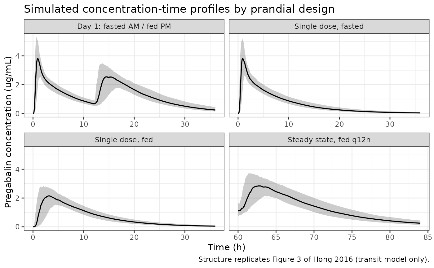
The absorption-phase contrast that motivated the paper is clearest with the two single-dose arms overlaid. The fasted profile rises to an early, sharp peak; the fed profile is flattened and delayed, and – the feature a first-order model cannot produce – its rise is concave rather than exponential-decay-shaped, because the gamma-density input rate increases over time before it falls.
sim |>
  filter(cohort %in% c("Single dose, fasted", "Single dose, fed"),
    time <= 12
  ) |>
  group_by(cohort, time) |>
  summarise(Q50 = quantile(Cc, 0.50), .groups = "drop") |>
  ggplot(aes(time, Q50, colour = cohort)) +
  geom_line(linewidth = 0.7) +
  labs(
    x = "Time (h)", y = "Median pregabalin concentration (ug/mL)",
    colour = NULL,
    title = "Absorption phase, fasted vs fed (typical 150 mg single dose)"
  ) +
  theme_bw() +
  theme(legend.position = "bottom")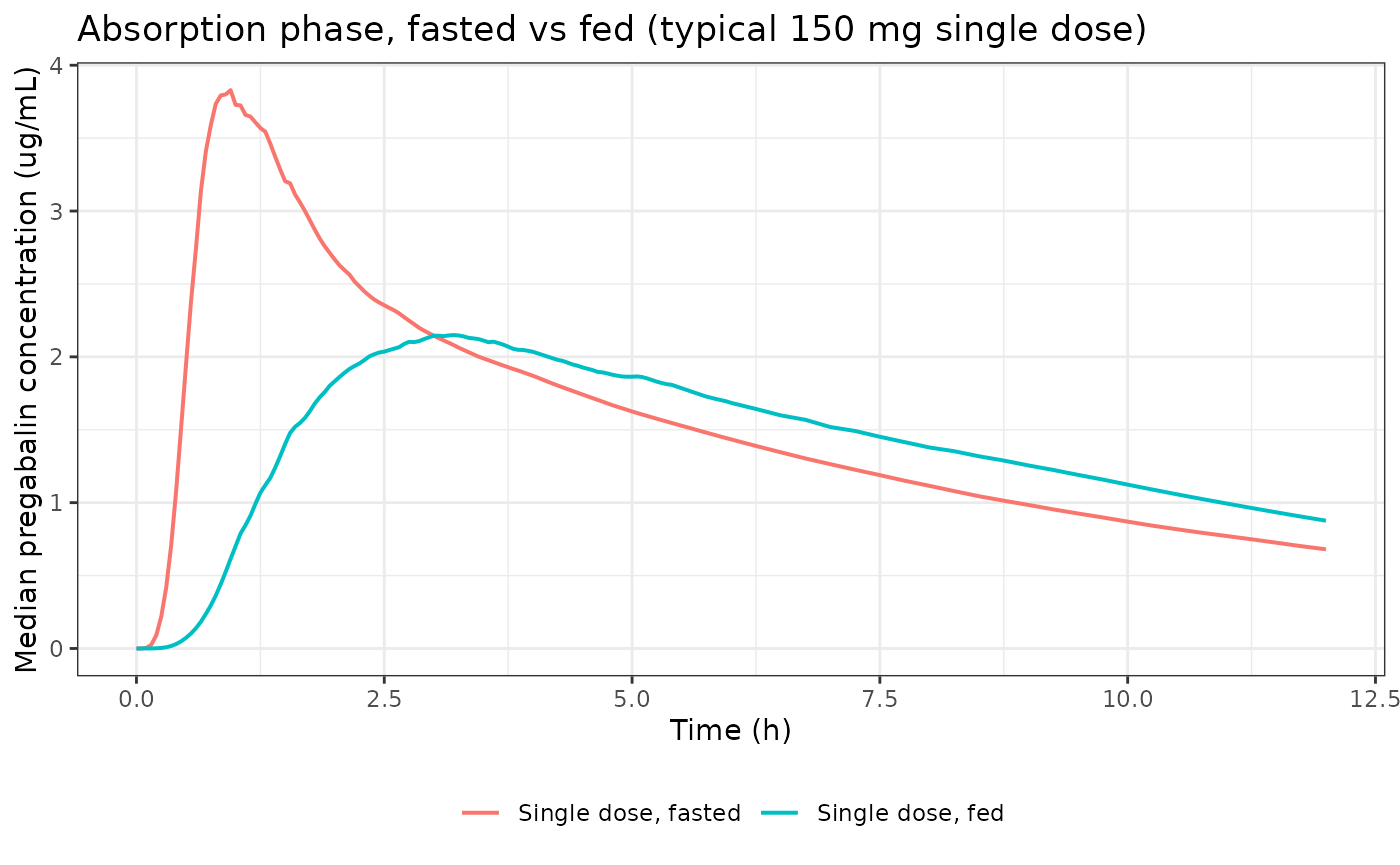
PKNCA validation
NCA is run on the two clean single-dose arms, where the fasted-versus-fed absorption contrast is unconfounded by accumulation.
sim_nca <- sim |>
  filter(cohort %in% c("Single dose, fasted", "Single dose, fed")) |>
  filter(!is.na(Cc)) |>
  select(id, time, Cc, cohort)

# Guarantee a time = 0 row per (id, cohort); for an extravascular dose the
# correct pre-dose value is 0. Without it PKNCA warns on every subject that the
# AUC interval starts before the first measurement.
sim_nca <- bind_rows(
  sim_nca,
  sim_nca |> distinct(id, cohort) |> mutate(time = 0, Cc = 0)
) |>
  distinct(id, cohort, time, .keep_all = TRUE) |>
  arrange(id, cohort, time)

conc_obj <- PKNCA::PKNCAconc(sim_nca, Cc ~ time | cohort + id)

dose_df <- events |>
  filter(evid == 1, cohort %in% c("Single dose, fasted", "Single dose, fed")) |>
  select(id, time, amt, cohort)

dose_obj <- PKNCA::PKNCAdose(dose_df, amt ~ time | cohort + id)

intervals <- data.frame(
  start = 0, end = Inf,
  cmax = TRUE, tmax = TRUE,
  auclast = TRUE, aucinf.obs = TRUE, half.life = TRUE
)

nca_res <- PKNCA::pk.nca(PKNCA::PKNCAdata(conc_obj, dose_obj,
  intervals = intervals
))

nca_wide <- as.data.frame(nca_res) |>
  select(cohort, id, PPTESTCD, PPORRES) |>
  tidyr::pivot_wider(names_from = PPTESTCD, values_from = PPORRES)

nca_wide |>
  group_by(cohort) |>
  summarise(
    `Cmax (ug/mL)` = median(cmax),
    `Tmax (h)` = median(tmax),
    `AUCinf (ug*h/mL)` = median(aucinf.obs),
    `t1/2 (h)` = median(half.life),
    .groups = "drop"
  ) |>
  rename("Arm" = cohort) |>
  knitr::kable(
    digits = 3,
    caption = "Median simulated NCA parameters after a single 150 mg dose."
)| Arm | Cmax (ug/mL) | Tmax (h) | AUCinf (ug*h/mL) | t1/2 (h) |
|---|---|---|---|---|
| Single dose, fasted | 4.048 | 1.000 | 24.188 | 5.442 |
| Single dose, fed | 2.226 | 3.125 | 23.805 | 5.479 |
Hong 2016 reports no NCA table – the paper’s own
exposure comparisons were made with linear-trapezoidal AUCs that it
explicitly declines to tabulate (“not shown in this report”). There is
therefore nothing to place in an ncaComparisonTable(), and
the NCA above characterises the packaged model rather than validating it
against published NCA. Validation instead uses the quantitative claims
the paper does state, below.
Structural gate: mass balance
For a linear model, CL/F x AUCinf must equal
Dose x F exactly, per subject. This is the one check that
the known transit() + f(depot) <- 0 failure
mode (a silent all-zero solve) cannot pass, and it also catches a dose
arriving twice. Both sides use the same drawn parameters, so the
residual is pure numerical error and a tight bound is appropriate.
cl_by_id <- sim |>
  group_by(id) |>
  summarise(cl = first(cl), .groups = "drop")

mb <- nca_wide |>
  left_join(cl_by_id, by = "id") |>
  mutate(ratio = cl * aucinf.obs / DOSE_MG)

stopifnot(nrow(mb) == 2L * N_ARM) # a zero-row join would pass vacuously
cat(sprintf(
  "mass-balance CL/F * AUCinf / Dose: min %.6f, max %.6f\n",
  min(mb$ratio), max(mb$ratio)
))
#> mass-balance CL/F * AUCinf / Dose: min 0.999859, max 1.001269
stopifnot(all(abs(mb$ratio - 1) < 0.01))
Published quantitative claims
Each row below is a number Hong 2016 states in prose or in a table, checked against the packaged model. Tolerances are absolute and set to half of the last printed digit, because the published values are rounded and no single percentage tolerance works across values printed to different precision.
ui <- rxode2::rxode(mod)
th <- setNames(ui$theta, names(ui$theta))

cl_t <- exp(th[["lcl"]])
mtt_fasted <- exp(th[["lmtt_fasted"]])
mtt_fed <- exp(th[["lmtt_fed"]])
ka_fasted <- exp(th[["lka_fasted"]])
ka_fed <- exp(th[["lka_fed"]])
nn <- exp(th[["lnn"]])

# Claim 1 is the strongest available: it is non-circular (the value appears in
# the Discussion, not in Table 5) and it constrains the intercept, the exponent
# and the 120 mL/min centring value simultaneously.
cl_at_107 <- cl_t * (107 / 120)^th[["e_crcl_cl"]]
ka_drop_pct <- 100 * (1 - ka_fed / ka_fasted)
mtt_gain <- mtt_fed - mtt_fasted
v_total <- exp(th[["lvc"]]) + exp(th[["lvp"]])

claims <- tibble::tribble(
  ~Claim, ~Source, ~Published, ~Model, ~Tol, ~Deviation,
  "CL/F of a typical subject at CLCR = 107 mL/min (L/h)",
  "Discussion", 5.89, cl_at_107, 0.005, FALSE,
  "Reduction in absorption rate constant when fed (%)",
  "Discussion", 87.5, ka_drop_pct, 0.05, FALSE,
  "Prolongation of mean transit time when fed (h)",
  "Discussion", 0.39, mtt_gain, 0.01, FALSE,
  "Apparent clearance CL/F of the final model (L/h)",
  "Table 4", 6.25, cl_t, 0.005, FALSE,
  "Number of transit compartments of the final model",
  "Table 4", 3.61, nn, 0.005, FALSE,
  "Total apparent volume V/F = V2/F + V3/F (L)",
  "Table 4", 44.9, v_total, 0.05, TRUE
) |>
  mutate(
    Diff = Model - Published,
    Pass = abs(Diff) <= Tol
  )

claims |>
  select(Claim, Source, Published, Model, Diff, Pass, Deviation) |>
  rename(
    "Published value" = Published, "Model value" = Model,
    "Difference" = Diff, "Known deviation" = Deviation
  ) |>
  knitr::kable(
    digits = 4,
    caption = paste(
      "Published claims from Hong 2016 checked against the packaged model.",
      "Tolerances are half of the last printed digit."
    )
)| Claim | Source | Published value | Model value | Difference | Pass | Known deviation |
|---|---|---|---|---|---|---|
| CL/F of a typical subject at CLCR = 107 mL/min (L/h) | Discussion | 5.89 | 5.8943 | 0.0043 | TRUE | FALSE |
| Reduction in absorption rate constant when fed (%) | Discussion | 87.50 | 87.4692 | -0.0308 | TRUE | FALSE |
| Prolongation of mean transit time when fed (h) | Discussion | 0.39 | 0.3850 | -0.0050 | TRUE | FALSE |
| Apparent clearance CL/F of the final model (L/h) | Table 4 | 6.25 | 6.2500 | 0.0000 | TRUE | FALSE |
| Number of transit compartments of the final model | Table 4 | 3.61 | 3.6100 | 0.0000 | TRUE | FALSE |
| Total apparent volume V/F = V2/F + V3/F (L) | Table 4 | 44.90 | 45.0000 | 0.1000 | FALSE | TRUE |
# Gate on every non-deviation row. The one flagged row is discussed below and
# is deliberately excluded rather than having its tolerance widened until it
# passes.
stopifnot(all(claims$Pass[!claims$Deviation]))
The total-volume row is a genuine, minor inconsistency within the paper, not a transcription error. Table 4 gives the final model’s V/F as 44.9 L with the footnote “sum of central volume and peripheral volume”, while Table 5 reports V2/F = 18.0 L and V3/F = 27.0 L, which sum to 45.0 L. The 0.1 L gap is consistent with Table 4 having been computed from unrounded estimates (e.g. 17.96 + 26.95 = 44.91) that Table 5 then rounded to three significant figures. The model uses the Table 5 values, which are the ones reported as the final estimates with precision and bootstrap intervals.
Dose superimposition
The paper implemented Shen 2012 dose superimposition (its reference
14) so that a dose whose absorption is incomplete still contributes
input after the next dose is given. rxode2’s transit()
builtin instead restarts the gamma input at each dose. This is a real
structural difference, so it has to be shown to be immaterial rather
than assumed to be.
It is immaterial here because absorption is fast relative to the 12 h
dosing interval. The Savic input is a gamma density with shape
NN + 1 and rate ktr = (NN + 1) / MTT, so the
fraction of a dose delivered by the time the next one arrives is a gamma
CDF.
frac_absorbed_at_tau <- function(mtt, tau = 12) {
  ktr <- (nn + 1) / mtt
  pgamma(tau, shape = nn + 1, rate = ktr)
}

fed_frac <- frac_absorbed_at_tau(mtt_fed) # the slower of the two states
cat(sprintf(
  "Fraction of a dose delivered by tau = 12 h: fasted %.10f, fed %.10f\n",
  frac_absorbed_at_tau(mtt_fasted), fed_frac
))
#> Fraction of a dose delivered by tau = 12 h: fasted 1.0000000000, fed 1.0000000000

# Deterministic (no cohort draw), so an exact bound is appropriate.
stopifnot(fed_frac > 1 - 1e-9)
Even in the fed state, which has the longer mean transit time of the two, the input is complete to within one part in a billion before the next dose arrives. Restarting rather than superimposing the gamma input therefore has no numerical consequence at this paper’s 12 h interval. A user who shortens the interval to a few hours, or who reuses these absorption parameters for a drug or formulation with a much longer MTT, would need to revisit this.
Food effect on exposure and on rate
The paper’s reason for not modelling a bioavailability change with food is that its trapezoidal AUC comparison found none. The packaged model should therefore shift the rate of absorption substantially while leaving the extent untouched.
The gate below is deliberately run on the
typical-value profile (zeroRe(),
creatinine clearance held at the 120 mL/min reference) rather than on
the cohort medians. Comparing medians of two independently drawn cohorts
would put roughly a 2.6% standard error on the AUC ratio, so any
tolerance tight enough to be meaningful would flicker between CI
machines that solve on different thread counts. With the random effects
zeroed the contrast is deterministic and the same on every machine, so
it can be asserted tightly and still go red if a food effect were ever
wired into F or cl.
typ <- rxode2::zeroRe(mod)

# Fine through absorption, coarse through the terminal phase; 168 h is many
# half-lives, so the trapezoidal integral is effectively AUCinf.
typ_times <- sort(unique(c(seq(0, 12, by = 0.01), seq(12, 168, by = 0.1))))

typical_profile <- function(fed) {
  ev <- data.frame(
    id = 1L,
    time = c(0, typ_times),
    amt = c(DOSE_MG, rep(NA_real_, length(typ_times))),
    evid = c(1L, rep(0L, length(typ_times))),
    cmt = c("depot", rep("central", length(typ_times))),
    FED = fed,
    CRCL = 120
  )
  rxode2::rxSolve(typ, ev, covsInterpolation = "locf") |> as.data.frame()
}

trapz <- function(x, y) sum(diff(x) * (head(y, -1) + tail(y, -1)) / 2)

p_fasted <- typical_profile(0)
#> ℹ omega/sigma items treated as zero: 'etalcl', 'etalvc', 'etalmtt_fasted', 'etalmtt_fed', 'etalka'
p_fed <- typical_profile(1)
#> ℹ omega/sigma items treated as zero: 'etalcl', 'etalvc', 'etalmtt_fasted', 'etalmtt_fed', 'etalka'
stopifnot(nrow(p_fasted) > 100, nrow(p_fed) > 100)

auc_fasted <- trapz(p_fasted$time, p_fasted$Cc)
auc_fed <- trapz(p_fed$time, p_fed$Cc)
auc_ratio <- auc_fed / auc_fasted
cmax_ratio <- max(p_fed$Cc) / max(p_fasted$Cc)
tmax_ratio <- p_fed$time[which.max(p_fed$Cc)] /
  p_fasted$time[which.max(p_fasted$Cc)]

cat(sprintf(
  "typical-value fed/fasted ratios -- AUC0-168 %.6f, Cmax %.4f, Tmax %.4f\n",
  auc_ratio, cmax_ratio, tmax_ratio
))
#> typical-value fed/fasted ratios -- AUC0-168 1.000002, Cmax 0.5404, Tmax 2.9263

# Extent must be untouched: neither F nor cl depends on FED, so the only
# difference between the two integrals is solver/trapezoid error. Deterministic,
# hence a tight bound. This goes red if a food effect is ever added to F or cl.
stopifnot(abs(auc_ratio - 1) < 0.002)

# Rate effects are large -- ka falls 8-fold and MTT nearly doubles. Also
# deterministic here, but bounds are kept as magnitude claims rather than
# pinned to the realised values so they stay readable as statements of the
# paper's finding. Realised: Cmax ratio ~0.55, Tmax ratio ~3.1.
stopifnot(cmax_ratio < 0.85)
stopifnot(tmax_ratio > 1.8)

# The cohort medians are reported for context but deliberately NOT gated.
nca_wide |>
  group_by(cohort) |>
  summarise(
    `Median Cmax (ug/mL)` = median(cmax),
    `Median Tmax (h)` = median(tmax),
    `Median AUCinf (ug*h/mL)` = median(aucinf.obs),
    .groups = "drop"
  ) |>
  rename("Arm" = cohort) |>
  knitr::kable(
    digits = 3,
    caption = "Cohort medians (descriptive; the gate above uses typical values)."
)| Arm | Median Cmax (ug/mL) | Median Tmax (h) | Median AUCinf (ug*h/mL) |
|---|---|---|---|
| Single dose, fasted | 4.048 | 1.000 | 24.188 |
| Single dose, fed | 2.226 | 3.125 | 23.805 |
Exposure is unchanged while the peak is materially lower and materially later, which is the behaviour the paper describes and the clinical reason it cared: pregabalin’s common adverse events track peak concentration, so an absorption model that misplaces Cmax misstates the safety profile even when it gets AUC right.
Assumptions and deviations
Only the winning model is packaged. Table 4 lists six candidate structures. For the five rejected ones the paper reports only the number of parameters, the objective function value, CL/F and total V/F, which is not enough to reconstruct them. The paper’s central claim – that the transit model beats the first-order model by dAIC 497.3 and the Erlang model by dAIC 8.5 – is a model-selection result that cannot be reproduced without refitting to the original data, which are not public. It is recorded here as a claim of the source, not as a gate.
Dose superimposition is approximated. The source used the Shen 2012 NONMEM implementation of dose superimposition; rxode2’s
transit()restarts the gamma input at each dose. The “Dose superimposition” section above quantifies the difference as under one part in a billion at this paper’s 12 h interval and states when a user would need to revisit it.f(depot) <- 0is a known rxode2 hazard. The idiom that suppresses the dose bolus sotransit()is the sole input pathway silently returns an all-zero solve for some models at rxode2 5.1.x. This model was verified not to be affected, and the mass-balance gate above is the standing regression check; ratio-based checks are useless for this failure because they divide one zero by another and pass.Random effects are back-transformed from percent CV. Table 5 reports between-subject variability as CV% and the Methods state that variability entered exponentially, so
omega^2 = log(1 + CV^2). The alternative reading, that the printed CV% is the omega standard deviation directly, would inflate the MTT-fed variance from 0.513 to 0.671; the log-normal back-transform is the convention used throughout nlmixr2lib.Variability the paper did not estimate is absent, not invented. Table 5 marks between-subject variability on Q/F, V3/F and NN as “not estimated”, so the model carries no eta on those parameters.
The creatinine-clearance term must not be extrapolated to renal impairment. The cohort is 88 healthy young men with per-study mean CLCR of 110.8-132.8 mL/min. The paper devotes a Discussion section and Figure 4 to the point that, unlike Bockbrader 2011 and Shoji 2011, it finds no breakpoint at 107 mL/min above which CL/F plateaus – and attributes the difference to its small, homogeneous sample rather than to a real absence of the plateau. For renally impaired subjects,
Shoji_2011_pregabalinis the appropriate model in this package.Prandial detail is collapsed to one binary flag. Studies differed in meal type (regular or high-fat) and in dose timing relative to the meal (30 min or 4 h). The authors state that these distinctions “were not successfully modeled” and were “not significantly different or discernible”, so the model has a single fed-versus-fasted indicator and
FED_HIGHFATis deliberately unused despite study 4 giving a high-fat breakfast.Bioavailability is fixed to 1. Oral-only data cannot identify F; the paper folds it into the apparent parameters CL/F, V2/F, Q/F and V3/F and does not allow it to change with food.
Virtual covariate distribution. Creatinine clearance is drawn as Normal(120.0, 21.6) mL/min per Table 1’s pooled statistics and truncated to 70-190 mL/min. The paper publishes per-study means and standard deviations but not the individual values or the distributional shape.
Concentration units. The model returns ug/mL (equivalently mg/L) from a dose in mg and volumes in L. The paper tabulates assay lower limits of quantification in ng/mL (Table 3), which are 1000x the model’s units.