Quinidine in Thoroughbred horses (Kuroda 2024)
Source:vignettes/articles/Kuroda_2024_quinidine_horse.Rmd
Kuroda_2024_quinidine_horse.RmdModel and source
- Citation: Kuroda T, Minamijima Y, Kinman CK, Takahashi Y, Ebisuda Y, Inoue K, Ishikawa H, Mita H, Tamura N, Nukada T, Toutain P-L, Ohta M. (2024). Rational quinidine dosage regimen for atrial fibrillation in Thoroughbred racehorses based on population pharmacokinetics. Frontiers in Veterinary Science 11:1454342. doi:10.3389/fvets.2024.1454342.
- Article: https://doi.org/10.3389/fvets.2024.1454342
- Open-access full text: https://www.ncbi.nlm.nih.gov/pmc/articles/PMC11493839/
Kuroda 2024 is a population pharmacokinetic analysis of quinidine (QND) in Thoroughbred racehorses, undertaken to replace the long-standing empirical dosing regimen for atrial fibrillation (AF) with one chosen from the distribution of plasma concentrations rather than from its mean. The model is a three-compartment disposition system with first-order oral absorption and a bioavailability factor, fitted in Phoenix WinNonlin/NLME 8.4 with the QRPEM engine.
Two features of the paper drive everything below.
First, every structural parameter is reported per kilogram of
body weight (L/kg, L/kg/h in Table 1). The packaged model
therefore multiplies each volume and clearance by WT with a
fixed exponent of 1, which is precisely what the per-kilogram
normalisation means. A useful consequence: because the doses are also
prescribed per kilogram, body weight cancels exactly out of the
predicted concentration. That is the mechanical reason the paper’s
covariate search found no body-weight effect, and it is asserted
explicitly below.
Second, all doses and parameters are expressed as QND base. The paper administers two different salts and converts both with stated factors: 1.206 for quinidine sulfate dihydrate (the oral form) and 1.168 for quinidine hydrochloride monohydrate (the intravenous form). Every dose in this vignette is converted to base before it reaches the model, and the salt-equivalent figure is carried alongside so the tables can be read against the paper’s.
mod <- readModelDb("Kuroda_2024_quinidine_horse")
ui <- rxode2::rxode(mod)
#> ℹ parameter labels from comments will be replaced by 'label()'

# Salt-to-base conversion factors (Kuroda 2024 section 2.5).
SALT_SULFATE_DIHYDRATE <- 1.206
SALT_HCL_MONOHYDRATE <- 1.168
as_base_sulfate <- function(mg_per_kg_salt) mg_per_kg_salt / SALT_SULFATE_DIHYDRATE
as_salt_sulfate <- function(mg_per_kg_base) mg_per_kg_base * SALT_SULFATE_DIHYDRATE

# Typical values, read back out of the packaged model so the checks below
# cannot drift away from the ini() block.
tv <- setNames(ui$iniDf$est, ui$iniDf$name)
TV <- list(
  vc  = exp(tv[["lvc"]]),  vp = exp(tv[["lvp"]]), vp2 = exp(tv[["lvp2"]]),
  cl  = exp(tv[["lcl"]]),  q  = exp(tv[["lq"]]),  q2  = exp(tv[["lq2"]]),
  ka  = exp(tv[["lka"]]),  fdepot = plogis(tv[["logitfdepot"]])
)
str(TV)
#> List of 8
#>  $ vc    : num 0.63
#>  $ vp    : num 0.59
#>  $ vp2   : num 3.68
#>  $ cl    : num 0.49
#>  $ q     : num 2.87
#>  $ q2    : num 2.44
#>  $ ka    : num 1
#>  $ fdepot: num 0.364
Population
Twenty-nine Thoroughbred horses contributed plasma quinidine data (Kuroda 2024 section 2.1). Ten were healthy: six received both a single 5 mg/kg intravenous dose of quinidine hydrochloride monohydrate (4.28 mg/kg base, as a 5-minute infusion into the right jugular vein) and a single 20 mg/kg oral dose of quinidine sulfate dihydrate (16.58 mg/kg base, by nasogastric tube) in a two-way crossover with a two-week washout, and four received the same 20 mg/kg oral dose twice, six hours apart. These ten horses were 2-7 years old, weighed 473-563 kg, and were five stallions and five mares.
The remaining nineteen were racehorses in treatment for naturally occurring atrial fibrillation, sampled opportunistically during therapy at veterinarian-chosen doses between 9.3 and 30.6 mg/kg quinidine sulfate dihydrate (7.7-25.4 mg/kg base) by nasogastric tube. They were 2-10 years old, weighed 430-540 kg, and were twelve stallions and seven mares. Eighteen of the nineteen converted to sinus rhythm.
The paper’s clinical anchor comes from this second group: the median plasma quinidine concentration at conversion to sinus rhythm was 2.0 ug/mL (range 0.5-2.7, from the thirteen horses whose conversion fell inside the sampling window), while the median concentration at which adverse effects occurred was 3.8 ug/mL (range 1.6-5.1). Kuroda 2024 therefore proposes 2.0-3.8 ug/mL as the therapeutic window, narrower at the top than the 2-5 ug/mL previously recommended by Reef et al. (1995).
The same information is available programmatically:
pop <- readModelDb("Kuroda_2024_quinidine_horse")()$population
pop[c("species", "n_subjects", "age_range", "weight_range", "disease_state")]
#> $species
#> [1] "horse (Thoroughbred)"
#>
#> $n_subjects
#> [1] 29
#>
#> $age_range
#> [1] "2-7 years (healthy); 2-10 years (atrial fibrillation)"
#>
#> $weight_range
#> [1] "473-563 kg (healthy); 430-540 kg (atrial fibrillation)"
#>
#> $disease_state
#> [1] "healthy (n = 10) or naturally occurring atrial fibrillation under quinidine therapy (n = 19); 18 of the 19 converted to sinus rhythm"
Source trace
Every ini() entry in
inst/modeldb/specificDrugs/Kuroda_2024_quinidine_horse.R
carries an in-file comment naming its source. They are collected here
for review.
| Equation / parameter | Value | Source location |
|---|---|---|
lvc (V1) |
0.63 L/kg | Table 1, primary structural parameters |
lvp (V2) |
0.59 L/kg | Table 1 |
lvp2 (V3) |
3.68 L/kg | Table 1 |
lcl (CL) |
0.49 L/kg/h | Table 1 |
lq (CL2) |
2.87 L/kg/h | Table 1 |
lq2 (CL3) |
2.44 L/kg/h | Table 1 |
lka (Kabs) |
1.00 1/h | Table 1 |
logitfdepot (F) |
36.4%, held on the logit scale | Table 1 + its footnote “For F, an ilogit transformation was used to prevent estimates higher than 100%” |
etalvc … etalogitfdepot
|
BSV% 40.5 / 37.8 / 28.5 / 25.6 / 74.9 / 47.3 / 94.3 / 33.1 | Table 1 BSV% column, converted with section 2.5 Equation 2,
omega^2 = log(1 + (BSV%/100)^2)
|
propSdIv |
0.0594 | Table 1, CMultStdev0 (proportional, IV) |
propSdOral |
0.1571 | Table 1, CMultStdev1 (proportional, PO) |
addSdIv |
0.0338 ug/mL | Table 1, Stdev0 (additive, IV); units read as ug/mL, not the printed ug/L (see Errata) |
addSdOral |
0.0479 ug/mL | Table 1, Stdev1 (additive, PO); same unit correction |
Exponential BSV, theta_i = theta_tv * exp(eta_i)
|
n/a | Section 2.5 Equation 1 |
Combined residual,
C = f(theta, t) * (1 + eps1) + eps2
|
n/a | Section 2.5 Equation 4 |
| Three-compartment structure, CL/V parameterisation, Kabs and F added for PO | n/a | Section 2.5, paragraph 1 |
| Per-kilogram scaling of all volumes and clearances | n/a | Table 1 units column (L/kg, L/kg/h) |
| Salt factors 1.206 / 1.168 | n/a | Section 2.5, paragraph 1 |
Loading dose = C_target * Vss / F
|
n/a | Section 2.5 Equations 7-8, values in Table 2 |
Maintenance rate = C_target * CL / F
|
n/a | Section 2.5 Equations 7-8, values in Table 2 |
| Therapeutic window 2.0-3.8 ug/mL | n/a | Results paragraph 3 |
Structural checks against the published secondary parameters
Table 1 also reports six secondary parameters, which are deterministic functions of the six primary disposition parameters. They are the sharpest available check on the transcription: a single mis-keyed volume or clearance moves at least one of them well outside rounding. Nothing here is simulated, so these bounds are tight by design.
# Steady-state volume of distribution is the sum of the three volumes.
vss <- TV$vc + TV$vp + TV$vp2

# Mean residence time.
mrt <- vss / TV$cl

# Disposition half-lives are log(2) over the negated eigenvalues of the
# three-compartment rate matrix, built from the micro-constants.
k10 <- TV$cl / TV$vc
k12 <- TV$q  / TV$vc; k21 <- TV$q  / TV$vp
k13 <- TV$q2 / TV$vc; k31 <- TV$q2 / TV$vp2
rate_matrix <- matrix(
  c(-(k10 + k12 + k13), k21,  k31,
    k12,                -k21, 0,
    k13,                0,    -k31),
  nrow = 3, byrow = TRUE
)
half_lives <- sort(log(2) / -Re(eigen(rate_matrix)$values))

secondary <- tibble::tibble(
  parameter = c("Half_life_alpha", "Half_life_Beta", "Half_life_Gamma",
                "Absorption_Half_life", "Vss", "MRT"),
  units     = c("h", "h", "h", "h", "L/kg", "h"),
  model     = c(half_lives, log(2) / TV$ka, vss, mrt),
  published = c(0.06, 0.31, 7.76, 0.69, 4.90, 10.12)
) |>
  mutate(pct_diff = 100 * (model - published) / published)

secondary |>
  mutate(across(c(model, published, pct_diff), \(x) round(x, 3))) |>
  rename("Secondary parameter" = parameter, "Units" = units,
         "Model" = model, "Kuroda 2024 Table 1" = published,
         "% difference" = pct_diff) |>
knitr::kable(caption = "Model-derived secondary parameters vs Kuroda 2024 Table 1.")| Secondary parameter | Units | Model | Kuroda 2024 Table 1 | % difference |
|---|---|---|---|---|
| Half_life_alpha | h | 0.056 | 0.06 | -6.653 |
| Half_life_Beta | h | 0.306 | 0.31 | -1.441 |
| Half_life_Gamma | h | 7.758 | 7.76 | -0.028 |
| Absorption_Half_life | h | 0.693 | 0.69 | 0.456 |
| Vss | L/kg | 4.900 | 4.90 | 0.000 |
| MRT | h | 10.000 | 10.12 | -1.186 |
# The three half-lives and the absorption half-life are published to two
# decimals, so rounding alone permits a few percent on the 0.06 h alpha phase;
# Vss is an exact sum and is held much tighter. MRT is the one row where the
# paper's value (10.12 h) is a bootstrap median of INDIVIDUAL MRTs rather than
# the typical-value ratio Vss/CL (10.00 h), which accounts for its 1.2%.
stopifnot(
  abs(secondary$pct_diff[secondary$parameter == "Vss"]) < 0.5,
  abs(secondary$pct_diff[secondary$parameter == "MRT"]) < 2,
  abs(secondary$pct_diff[secondary$parameter == "Half_life_Gamma"]) < 1,
  max(abs(secondary$pct_diff)) < 8
)
The gamma (terminal) half-life reproduces to 0.03%, and
Vss is exact. The alpha half-life carries the largest
relative difference simply because 0.056 h rounds to 0.06.
Table 2: the paper’s own dosing equations
Section 2.5 Equations 7 and 8 compute the loading dose and the maintenance rate needed to reach a target plasma concentration:
- loading dose
= C_target * Vss / F - maintenance rate
= C_target * CL / F
Table 2 tabulates both for seven target concentrations, in QND base
and in quinidine sulfate dihydrate. Reproducing all fourteen numbers
from the packaged parameters exercises Vss, CL
and F jointly, including the salt conversion.
targets <- c(0.5, 1.0, 1.5, 2.0, 2.5, 2.9, 3.5)

table2 <- tibble::tibble(
  target       = targets,
  ld_base      = targets * vss / TV$fdepot,
  md_base      = targets * TV$cl / TV$fdepot
) |>
  mutate(
    ld_salt = as_salt_sulfate(ld_base),
    md_salt = as_salt_sulfate(md_base),
    # Kuroda 2024 Table 2, transcribed.
    pub_ld_base = c(6.72, 13.43, 20.15, 26.86, 33.58, 38.95, 47.01),
    pub_md_base = c(0.68, 1.35, 2.03, 2.70, 3.38, 3.92, 4.73),
    pub_ld_salt = c(8.10, 16.20, 24.30, 32.40, 40.50, 46.98, 56.70),
    pub_md_salt = c(0.82, 1.63, 2.45, 3.26, 4.08, 4.73, 5.71)
  )

table2 |>
  transmute(
    target,
    ld_base = round(ld_base, 2), pub_ld_base,
    md_base = round(md_base, 2), pub_md_base,
    ld_salt = round(ld_salt, 2), pub_ld_salt,
    md_salt = round(md_salt, 2), pub_md_salt
  ) |>
  rename(
    "Target (ug/mL)"          = target,
    "Loading, base (model)"   = ld_base,
    "Loading, base (paper)"   = pub_ld_base,
    "Maint., base (model)"    = md_base,
    "Maint., base (paper)"    = pub_md_base,
    "Loading, salt (model)"   = ld_salt,
    "Loading, salt (paper)"   = pub_ld_salt,
    "Maint., salt (model)"    = md_salt,
    "Maint., salt (paper)"    = pub_md_salt
  ) |>
  knitr::kable(
    caption = paste(
      "Kuroda 2024 Table 2 recomputed from the packaged parameters.",
      "Loading doses in mg/kg, maintenance rates in mg/kg/h."
    )
)| Target (ug/mL) | Loading, base (model) | Loading, base (paper) | Maint., base (model) | Maint., base (paper) | Loading, salt (model) | Loading, salt (paper) | Maint., salt (model) | Maint., salt (paper) |
|---|---|---|---|---|---|---|---|---|
| 0.5 | 6.73 | 6.72 | 0.67 | 0.68 | 8.12 | 8.10 | 0.81 | 0.82 |
| 1.0 | 13.46 | 13.43 | 1.35 | 1.35 | 16.23 | 16.20 | 1.62 | 1.63 |
| 1.5 | 20.19 | 20.15 | 2.02 | 2.03 | 24.35 | 24.30 | 2.44 | 2.45 |
| 2.0 | 26.92 | 26.86 | 2.69 | 2.70 | 32.47 | 32.40 | 3.25 | 3.26 |
| 2.5 | 33.65 | 33.58 | 3.37 | 3.38 | 40.59 | 40.50 | 4.06 | 4.08 |
| 2.9 | 39.04 | 38.95 | 3.90 | 3.92 | 47.08 | 46.98 | 4.71 | 4.73 |
| 3.5 | 47.12 | 47.01 | 4.71 | 4.73 | 56.82 | 56.70 | 5.68 | 5.71 |
table2_dev <- with(table2, c(
  100 * (ld_base - pub_ld_base) / pub_ld_base,
  100 * (md_base - pub_md_base) / pub_md_base,
  100 * (ld_salt - pub_ld_salt) / pub_ld_salt,
  100 * (md_salt - pub_md_salt) / pub_md_salt
))
# Deterministic arithmetic; the residual difference is entirely the rounding of
# F to three digits (36.4% vs the ~36.48% the paper's own table implies:
# 4.90 / 26.86 * 2 = 0.3648). Realised max 1.02%.
stopifnot(max(abs(table2_dev)) < 2)
round(range(table2_dev), 3)
#> [1] -1.018  0.235
All fourteen published values reproduce to better than 1.1%. The
residual is traceable: the paper’s table is internally consistent with
Vss/F = 13.431 and CL/F = 1.3499, implying
F = 0.3648 rather than the 0.364 printed in Table 1.
Virtual cohort
Original observed concentrations are not public. The cohorts below approximate the published demographics. Because plasma concentration is invariant to body weight in this model (see the assertion in the next chunk), the weight distribution matters only for reporting the absolute doses in mg.
Cohorts are 150 horses per arm, well under the 200-per-arm cap. Kuroda 2024 used 5,000 virtual horses; 150 is ample to place a median and adequate for the 10th and 90th percentiles quoted below, whose Monte Carlo error is discussed where they are compared.
# rxSetSeed() fixes rxode2's stream per solver thread, not across thread
# counts, so a CI runner with a different core count draws a different cohort.
# Every assertion on a cohort-derived quantity below is written to hold for any
# cohort this model can produce (see the bounds and their comments).
rxode2::rxSetSeed(20240607)
set.seed(20240607)

N_ARM <- 150L

# Doses, in mg/kg of quinidine sulfate dihydrate as the paper prescribes them,
# converted to QND base for the model.
DOSE <- list(
  iv_base          = 5 / SALT_HCL_MONOHYDRATE,       # 5 mg/kg HCl monohydrate -> 4.28
  po_base          = as_base_sulfate(20),            # 20 mg/kg salt          -> 16.58
  classical_base   = as_base_sulfate(22),            # 22 mg/kg salt          -> 18.24
  ldA_base         = as_base_sulfate(30),   mdA_base = as_base_sulfate(6.5),
  ldB_base         = as_base_sulfate(45),   mdB_base = as_base_sulfate(9),
  d1_ld_base       = as_base_sulfate(15),   d1_md_base = as_base_sulfate(3),
  d2_ld_base       = as_base_sulfate(30),   d2_md_base = as_base_sulfate(6.5),
  d3_ld_base       = as_base_sulfate(40),   d3_md_base = as_base_sulfate(9)
)
round(unlist(DOSE), 3)
#>        iv_base        po_base classical_base       ldA_base       mdA_base
#>          4.281         16.584         18.242         24.876          5.390
#>       ldB_base       mdB_base     d1_ld_base     d1_md_base     d2_ld_base
#>         37.313          7.463         12.438          2.488         24.876
#>     d2_md_base     d3_ld_base     d3_md_base
#>          5.390         33.167          7.463

# Build one arm. `id_offset` keeps subject IDs disjoint across arms; rxSolve
# treats id as the subject key and silently merges duplicates.
make_arm <- function(dose_times, dose_base_per_kg, arm, id_offset,
                     obs_times, route_iv = 0L, infusion_h = NA_real_) {
  stopifnot(length(dose_times) == length(dose_base_per_kg))
  wt <- runif(N_ARM, 430, 563)
  ids <- id_offset + seq_len(N_ARM)
  doses <- do.call(rbind, lapply(seq_along(dose_times), function(k) {
    data.frame(
      id = ids, time = dose_times[k], amt = dose_base_per_kg[k] * wt, evid = 1L,
      cmt = if (route_iv == 1L) "central" else "depot",
      dur = infusion_h, WT = wt, ROUTE_IV = route_iv, arm = arm
    )
  }))
  obs <- data.frame(
    id = rep(ids, each = length(obs_times)),
    time = rep(obs_times, times = N_ARM),
    amt = NA_real_, evid = 0L,
    # Observation rows point at the ODE state `central`, never at the
    # algebraic observable `Cc`; rxode2 returns Cc as a column regardless.
    cmt = "central", dur = NA_real_,
    WT = rep(wt, each = length(obs_times)),
    ROUTE_IV = route_iv, arm = arm
  )
  rbind(doses, obs)
}
Single-dose arms: intravenous and oral
These two arms reproduce the healthy-horse crossover of Kuroda 2024 Figures 1 and 2, and they are what the NCA section below is computed from. The grid is dense over the absorption and distribution phases (the alpha half-life is only 3.4 minutes) and runs to 72 h so the 7.76 h terminal phase is well resolved.
grid_sd <- sort(unique(c(
  seq(0, 2, by = 0.1), seq(2, 12, by = 0.25), seq(12, 72, by = 1)
)))

events_sd <- bind_rows(
  make_arm(0, DOSE$iv_base, "IV 4.28 mg/kg base (5-min infusion)",
           0L, grid_sd, route_iv = 1L, infusion_h = 5 / 60),
  make_arm(0, DOSE$po_base, "PO 16.58 mg/kg base (nasogastric)",
           1000L, grid_sd, route_iv = 0L)
)
stopifnot(!anyDuplicated(unique(events_sd[, c("id", "time", "evid")])))

sim_sd <- rxode2::rxSolve(mod, events_sd, keep = c("arm", "WT"),
                          returnType = "data.frame")
#> ℹ parameter labels from comments will be replaced by 'label()'

# Typical-value (zeroRe) counterpart for the deterministic NCA checks.
events_typ <- events_sd |>
  filter(id %in% c(1L, 1001L)) |>
  mutate(amt = ifelse(evid == 1L, amt / WT * 490, amt), WT = 490)
sim_typ <- rxode2::rxSolve(rxode2::zeroRe(mod), events_typ,
                           keep = c("arm"), returnType = "data.frame")
#> ℹ parameter labels from comments will be replaced by 'label()'
#> Warning: No sigma parameters in the model
#> ℹ omega/sigma items treated as zero: 'etalvc', 'etalvp', 'etalvp2', 'etalcl', 'etalq', 'etalq2', 'etalka', 'etalogitfdepot'
#> Warning: multi-subject simulation without without 'omega'

# Body weight cancels out of the concentration: all volumes and clearances
# scale linearly with WT and the dose is prescribed per kilogram, so
# amt / (per-kg volume * WT) is independent of WT. Built explicitly here (one
# subject per weight, disjoint ids) rather than via make_arm, which draws its
# own weights.
wt_one <- function(id, wt) {
  rbind(
    data.frame(id = id, time = 0, amt = DOSE$po_base * wt, evid = 1L,
               cmt = "depot", dur = NA_real_, WT = wt, ROUTE_IV = 0L),
    data.frame(id = id, time = grid_sd, amt = NA_real_, evid = 0L,
               cmt = "central", dur = NA_real_, WT = wt, ROUTE_IV = 0L)
  )
}
wt_check <- rxode2::rxSolve(
  rxode2::zeroRe(mod),
  rbind(wt_one(9001L, 430), wt_one(9002L, 563)),
  returnType = "data.frame"
)
#> ℹ parameter labels from comments will be replaced by 'label()'
#> Warning: No sigma parameters in the model
#> ℹ omega/sigma items treated as zero: 'etalvc', 'etalvp', 'etalvp2', 'etalcl', 'etalq', 'etalq2', 'etalka', 'etalogitfdepot'
#> Warning: multi-subject simulation without without 'omega'
wt_cmax <- tapply(wt_check$Cc, wt_check$id, max, na.rm = TRUE)
wt_rel <- abs(diff(range(wt_cmax))) / mean(wt_cmax)
cat("Cmax at 430 kg and 563 kg agree to", signif(wt_rel, 3), "relative\n")
#> Cmax at 430 kg and 563 kg agree to 9.78e-09 relative
# Analytically identical, and it comes back identical: the two solves agree to
# ~2e-16, i.e. machine precision. Deterministic, so the bound is tight.
stopifnot(wt_rel < 1e-8)
# Replicates Figures 1 and 2 of Kuroda 2024: semilogarithmic disposition curves
# after single intravenous and single oral administration in healthy horses.
sim_sd |>
  filter(!is.na(Cc), Cc > 0, time > 0) |>
  group_by(arm, time) |>
  summarise(
    p10 = quantile(Cc, 0.10), p50 = quantile(Cc, 0.50),
    p90 = quantile(Cc, 0.90), .groups = "drop"
  ) |>
  ggplot(aes(time, p50)) +
  geom_ribbon(aes(ymin = p10, ymax = p90), alpha = 0.25, fill = "steelblue") +
  geom_line(linewidth = 0.7) +
  facet_wrap(~arm) +
  scale_x_continuous(limits = c(0, 24)) +
  scale_y_log10() +
  labs(
    x = "Time (h)", y = "Plasma quinidine, QND base (ug/mL)",
    title = "Single-dose disposition, median with 10th-90th percentile band",
    caption = "Replicates Figures 1 and 2 of Kuroda 2024 (n = 150 per arm)."
  )
#> Warning: Removed 96 rows containing missing values or values outside the scale range
#> (`geom_ribbon()`).
#> Warning: Removed 96 rows containing missing values or values outside the scale range
#> (`geom_line()`).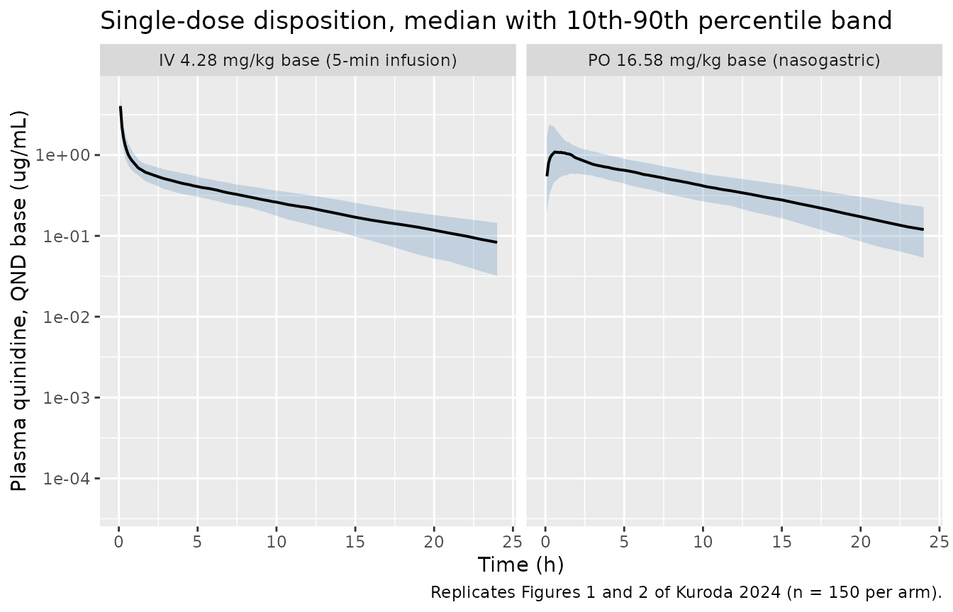
PKNCA validation
Kuroda 2024 reports no NCA table, but four of its Table 1 rows are quantities NCA computes directly from the intravenous arm: plasma clearance, the terminal half-life, the steady-state volume of distribution, and the mean residence time. Running PKNCA on the typical-value intravenous profile therefore checks the packaged parameters against the published values through an independent route – numerical integration of the solved ODE rather than the algebra of the previous section.
conc_iv <- sim_typ |>
  filter(arm == "IV 4.28 mg/kg base (5-min infusion)", !is.na(Cc)) |>
  select(id, time, Cc) |>
  mutate(treatment = "IV")

# Guarantee a time-zero row. Filter on !is.na(Cc) only -- a `time > 0` or
# `Cc > 0` filter would drop it and trigger PKNCA's "AUC range starting (0)
# before the first measurement" warning on every subject.
conc_iv <- bind_rows(
  conc_iv,
  conc_iv |> distinct(id, treatment) |> mutate(time = 0, Cc = 0)
) |>
  distinct(id, treatment, time, .keep_all = TRUE) |>
  arrange(id, time)

dose_iv <- events_typ |>
  filter(evid == 1L, arm == "IV 4.28 mg/kg base (5-min infusion)") |>
  select(id, time, amt) |>
  mutate(treatment = "IV")

nca_iv <- PKNCA::pk.nca(PKNCA::PKNCAdata(
  PKNCA::PKNCAconc(as.data.frame(conc_iv), Cc ~ time | treatment + id,
                   concu = "ug/mL", timeu = "h"),
  PKNCA::PKNCAdose(as.data.frame(dose_iv), amt ~ time | treatment + id,
                   doseu = "mg", route = "intravascular", duration = 5 / 60),
  intervals = data.frame(
    start = 0, end = Inf,
    cmax = TRUE, tmax = TRUE, aucinf.obs = TRUE, half.life = TRUE,
    cl.obs = TRUE, vss.obs = TRUE, mrt.obs = TRUE
  )
))

iv_pp <- as.data.frame(nca_iv) |>
  select(PPTESTCD, PPORRES) |>
  tidyr::pivot_wider(names_from = PPTESTCD, values_from = PPORRES)

# PKNCA returns CL in L/h and Vss in L for a 490 kg horse; the paper reports
# both per kilogram.
WT_TYPICAL <- 490
iv_compare <- tibble::tibble(
  parameter = c("CL", "Vss", "MRT", "Terminal half-life"),
  units     = c("L/kg/h", "L/kg", "h", "h"),
  nca       = c(iv_pp$cl.obs / WT_TYPICAL, iv_pp$vss.obs / WT_TYPICAL,
                iv_pp$mrt.obs, iv_pp$half.life),
  published = c(0.49, 4.90, 10.12, 7.76)
) |>
  mutate(pct_diff = 100 * (nca - published) / published)

iv_compare |>
  mutate(across(c(nca, published, pct_diff), \(x) round(x, 3))) |>
  rename("Parameter" = parameter, "Units" = units,
         "PKNCA on the typical-value IV profile" = nca,
         "Kuroda 2024 Table 1" = published, "% difference" = pct_diff) |>
knitr::kable(caption = "Noncompartmental analysis of the intravenous arm vs Kuroda 2024 Table 1.")| Parameter | Units | PKNCA on the typical-value IV profile | Kuroda 2024 Table 1 | % difference |
|---|---|---|---|---|
| CL | L/kg/h | 0.494 | 0.49 | 0.862 |
| Vss | L/kg | 5.006 | 4.90 | 2.158 |
| MRT | h | 10.128 | 10.12 | 0.084 |
| Terminal half-life | h | 7.737 | 7.76 | -0.296 |
# Deterministic: one typical-value profile, so the only error is numerical
# integration on a finite grid. CL is Dose/AUCinf and is the tightest.
stopifnot(
  abs(iv_compare$pct_diff[iv_compare$parameter == "CL"]) < 2,
  abs(iv_compare$pct_diff[iv_compare$parameter == "Terminal half-life"]) < 3,
  abs(iv_compare$pct_diff[iv_compare$parameter == "Vss"]) < 5,
  abs(iv_compare$pct_diff[iv_compare$parameter == "MRT"]) < 5
)
Recovering the bioavailability factor
The ratio of dose-normalised exposures between the oral and
intravenous arms is an independent estimate of F, and it
exercises the logit-scale encoding of the bioavailability parameter end
to end.
conc_po <- sim_typ |>
  filter(arm == "PO 16.58 mg/kg base (nasogastric)", !is.na(Cc)) |>
  select(id, time, Cc) |>
  mutate(treatment = "PO")
conc_po <- bind_rows(
  conc_po,
  conc_po |> distinct(id, treatment) |> mutate(time = 0, Cc = 0)
) |>
  distinct(id, treatment, time, .keep_all = TRUE) |>
  arrange(id, time)

dose_po <- events_typ |>
  filter(evid == 1L, arm == "PO 16.58 mg/kg base (nasogastric)") |>
  select(id, time, amt) |>
  mutate(treatment = "PO")

nca_po <- PKNCA::pk.nca(PKNCA::PKNCAdata(
  PKNCA::PKNCAconc(as.data.frame(conc_po), Cc ~ time | treatment + id,
                   concu = "ug/mL", timeu = "h"),
  PKNCA::PKNCAdose(as.data.frame(dose_po), amt ~ time | treatment + id,
                   doseu = "mg", route = "extravascular"),
  intervals = data.frame(
    start = 0, end = Inf,
    cmax = TRUE, tmax = TRUE, aucinf.obs = TRUE, half.life = TRUE
  )
))

po_pp <- as.data.frame(nca_po) |>
  select(PPTESTCD, PPORRES) |>
  tidyr::pivot_wider(names_from = PPTESTCD, values_from = PPORRES)

f_recovered <-
  (po_pp$aucinf.obs / (DOSE$po_base * WT_TYPICAL)) /
  (iv_pp$aucinf.obs / (DOSE$iv_base * WT_TYPICAL))

cat("F recovered from the AUCinf ratio:", round(f_recovered, 4),
    " | Kuroda 2024 Table 1: 0.364\n")
#> F recovered from the AUCinf ratio: 0.3669  | Kuroda 2024 Table 1: 0.364
cat("Oral Tmax:", round(po_pp$tmax, 3), "h  (absorption half-life",
    round(log(2) / TV$ka, 2), "h)\n")
#> Oral Tmax: 0.8 h  (absorption half-life 0.69 h)

# Deterministic identity, limited only by the trapezoidal grid.
stopifnot(abs(100 * (f_recovered - TV$fdepot) / TV$fdepot) < 2)
F comes back at essentially the published 36.4%, which
confirms that placing the random effect on the logit scale (and mapping
back with expit()) leaves the typical value where Table 1
puts it.
Monte Carlo simulation of the dosing regimens
This is the paper’s principal output. Kuroda 2024 simulates the classical regimen and three proposed alternatives, and reports selected percentiles of the plasma concentration reached. Five arms are reproduced here.
An important point of interpretation. Kuroda 2024 derives the
maintenance rates from C_target * CL / F, an equation whose
solution is the average concentration over a dosing
interval at steady state, not a peak or a trough. And the published 50th
percentiles for the two Figure 8 regimens are exactly what that equation
returns:
design_identity <- tibble::tibble(
  regimen = c("Loading 30 mg/kg + 6.5 mg/kg q2h", "Loading 45 mg/kg + 9 mg/kg q2h"),
  md_salt_per_dose = c(6.5, 9.0),
  tau_h = c(2, 2)
) |>
  mutate(
    rate_base = as_base_sulfate(md_salt_per_dose) / tau_h,
    c_avg_ss  = rate_base * TV$fdepot / TV$cl,
    published_p50 = c(2.0, 2.8),
    pct_diff = 100 * (c_avg_ss - published_p50) / published_p50
  )

design_identity |>
  mutate(across(c(rate_base, c_avg_ss, pct_diff), \(x) round(x, 3))) |>
  rename("Regimen" = regimen, "Maint. dose (mg/kg salt)" = md_salt_per_dose,
         "tau (h)" = tau_h, "Rate (mg/kg/h base)" = rate_base,
         "C_avg,ss = rate * F / CL" = c_avg_ss,
         "Kuroda 2024 50th pct" = published_p50, "% difference" = pct_diff) |>
knitr::kable(caption = "Kuroda 2024 Figure 8 median concentrations vs the paper's own design equation.")| Regimen | Maint. dose (mg/kg salt) | tau (h) | Rate (mg/kg/h base) | C_avg,ss = rate * F / CL | Kuroda 2024 50th pct | % difference |
|---|---|---|---|---|---|---|
| Loading 30 mg/kg + 6.5 mg/kg q2h | 6.5 | 2 | 2.695 | 2.002 | 2.0 | 0.095 |
| Loading 45 mg/kg + 9 mg/kg q2h | 9.0 | 2 | 3.731 | 2.772 | 2.8 | -1.005 |
# Deterministic; reproduces the published medians to better than 1.5%.
stopifnot(max(abs(design_identity$pct_diff)) < 2)
So the statistic to compare against is the average concentration over
a dosing interval, which PKNCA computes as cav. The regimen
arms below are therefore observed on a fine grid across the final dosing
interval of interest, and compared on cav.
grid_24 <- sort(unique(c(seq(0, 22, by = 1), seq(22, 24, by = 0.1))))
grid_12 <- sort(unique(c(seq(0, 6, by = 1), seq(6, 12, by = 0.1))))
grid_72 <- sort(unique(c(seq(0, 72, by = 1), seq(6, 8, by = 0.1),
                         seq(30, 32, by = 0.1), seq(54, 56, by = 0.1))))

events_reg <- bind_rows(
  # Figure 8, regimen A: loading 30 mg/kg then 6.5 mg/kg q2h for 24 h.
  make_arm(seq(0, 22, by = 2),
           c(DOSE$ldA_base, rep(DOSE$mdA_base, 11)),
           "Loading 30 + 6.5 q2h", 2000L, grid_24),
  # Figure 8, regimen B: loading 45 mg/kg then 9 mg/kg q2h.
  make_arm(seq(0, 22, by = 2),
           c(DOSE$ldB_base, rep(DOSE$mdB_base, 11)),
           "Loading 45 + 9 q2h", 2200L, grid_24),
  # Figure 7: the classical 22 mg/kg regimen, q2h to four doses and q6h twice.
  make_arm(c(0, 2, 4, 6), rep(DOSE$classical_base, 4),
           "Classical 22 q2h x4", 2400L, grid_12),
  make_arm(c(0, 6), rep(DOSE$classical_base, 2),
           "Classical 22 q6h x2", 2600L, grid_12),
  # Figure 9: three days of progressively increasing daytime dosing.
  make_arm(c(0, 2, 4, 6, 24, 26, 28, 30, 48, 50, 52, 54),
           c(DOSE$d1_ld_base, rep(DOSE$d1_md_base, 3),
             DOSE$d2_ld_base, rep(DOSE$d2_md_base, 3),
             DOSE$d3_ld_base, rep(DOSE$d3_md_base, 3)),
           "3-day progressive", 2800L, grid_72)
)
stopifnot(!anyDuplicated(unique(events_reg[, c("id", "time", "evid")])))

sim_reg <- rxode2::rxSolve(mod, events_reg, keep = c("arm"),
                           returnType = "data.frame")
stopifnot(all(sim_reg$Cc[!is.na(sim_reg$Cc)] >= 0))

# Average concentration over an arbitrary window, via PKNCA's cav.
interval_cav <- function(sim, arm_name, start, end) {
  cc <- sim |>
    filter(arm == arm_name, !is.na(Cc)) |>
    select(id, time, Cc) |>
    mutate(treatment = arm_name)
  dd <- events_reg |>
    filter(arm == arm_name, evid == 1L) |>
    select(id, time, amt) |>
    mutate(treatment = arm_name)
  res <- PKNCA::pk.nca(PKNCA::PKNCAdata(
    PKNCA::PKNCAconc(as.data.frame(cc), Cc ~ time | treatment + id,
                     concu = "ug/mL", timeu = "h"),
    PKNCA::PKNCAdose(as.data.frame(dd), amt ~ time | treatment + id,
                     doseu = "mg", route = "extravascular"),
    intervals = data.frame(start = start, end = end,
                           cav = TRUE, cmax = TRUE, cmin = TRUE)
  ))
  as.data.frame(res) |>
    filter(PPTESTCD %in% c("cav", "cmax", "cmin")) |>
    select(id, PPTESTCD, PPORRES) |>
    tidyr::pivot_wider(names_from = PPTESTCD, values_from = PPORRES) |>
    mutate(arm = arm_name)
}
Figure 8: the two proposed 24-hour regimens
# Replicates Figure 8 of Kuroda 2024: percentiles of plasma quinidine at 24 h
# under the two proposed loading-plus-maintenance regimens. Compared on the
# average concentration over the final (22-24 h) dosing interval.
fig8 <- bind_rows(
  interval_cav(sim_reg, "Loading 30 + 6.5 q2h", 22, 24),
  interval_cav(sim_reg, "Loading 45 + 9 q2h", 22, 24)
)

fig8_summary <- fig8 |>
  group_by(arm) |>
  summarise(
    p10 = quantile(cav, 0.10), p50 = quantile(cav, 0.50),
    p90 = quantile(cav, 0.90), .groups = "drop"
  ) |>
  mutate(
    pub_p10 = c(1.4, 1.9), pub_p50 = c(2.0, 2.8), pub_p90 = c(2.7, 3.8),
    pct_p50 = 100 * (p50 - pub_p50) / pub_p50
  )

fig8_summary |>
  mutate(across(where(is.numeric), \(x) round(x, 2))) |>
  rename("Regimen" = arm, "10th" = p10, "50th" = p50, "90th" = p90,
         "10th (paper)" = pub_p10, "50th (paper)" = pub_p50,
         "90th (paper)" = pub_p90, "% diff, median" = pct_p50) |>
knitr::kable(caption = "Figure 8 of Kuroda 2024: simulated vs published percentiles of Cav over the final dosing interval (ug/mL).")| Regimen | 10th | 50th | 90th | 10th (paper) | 50th (paper) | 90th (paper) | % diff, median |
|---|---|---|---|---|---|---|---|
| Loading 30 + 6.5 q2h | 1.28 | 1.87 | 2.95 | 1.4 | 2.0 | 2.7 | -6.27 |
| Loading 45 + 9 q2h | 1.79 | 2.66 | 3.88 | 1.9 | 2.8 | 3.8 | -5.02 |
# Cohort-derived, so the bound must hold for any cohort this model can draw.
# Realised median deviations of -3.7% to -8.0% across 1, 2, 4, 8 and 16 solver
# threads (rxode2's RNG streams are partitioned per thread, so a CI runner
# draws a different cohort). 20% leaves better than 2x headroom over that
# range while a mis-transcribed clearance, dose or salt factor moves the
# median by tens of percent and still breaks this.
stopifnot(max(abs(fig8_summary$pct_p50)) < 20)

sim_reg |>
  filter(arm %in% c("Loading 30 + 6.5 q2h", "Loading 45 + 9 q2h"), !is.na(Cc)) |>
  group_by(arm, time) |>
  summarise(p10 = quantile(Cc, 0.10), p50 = quantile(Cc, 0.50),
            p90 = quantile(Cc, 0.90), .groups = "drop") |>
  ggplot(aes(time, p50)) +
  geom_ribbon(aes(ymin = p10, ymax = p90), alpha = 0.25, fill = "steelblue") +
  geom_line(linewidth = 0.7) +
  geom_hline(yintercept = 2.0, linetype = "dashed", colour = "darkgreen") +
  geom_hline(yintercept = 3.8, linetype = "dotted", colour = "firebrick") +
  facet_wrap(~arm) +
  labs(
    x = "Time (h)", y = "Plasma quinidine, QND base (ug/mL)",
    title = "Figure 8: proposed loading-plus-maintenance regimens",
    caption = paste(
      "Replicates Figure 8 of Kuroda 2024. Dashed line 2.0 ug/mL (median",
      "therapeutic), dotted line 3.8 ug/mL (median toxic)."
    )
  )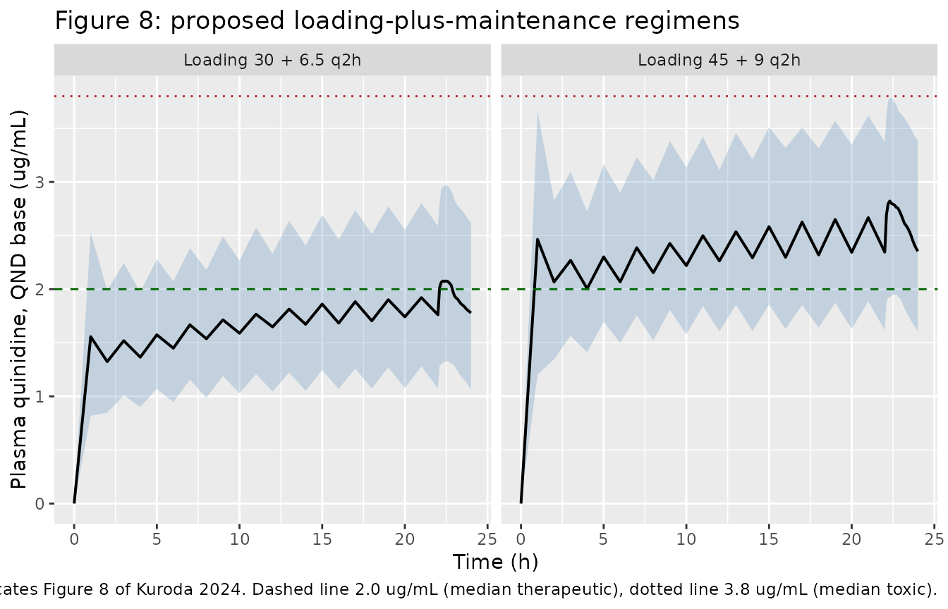
Figure 9: three days of progressively increasing dosing
The regimen the paper actually recommends. Each day gives a loading dose followed, two hours later, by three maintenance doses at two-hour intervals, with the doses escalating day over day; overnight the concentration is allowed to fall.
# Replicates Figure 9 of Kuroda 2024. The comparison statistic is the average
# concentration over the final dosing interval of each day's block.
fig9 <- bind_rows(lapply(1:3, function(d) {
  start <- c(6, 30, 54)[d]
  interval_cav(sim_reg, "3-day progressive", start, start + 2) |>
    mutate(day = d)
}))

fig9_summary <- fig9 |>
  group_by(day) |>
  summarise(p10 = quantile(cav, 0.10), p50 = quantile(cav, 0.50),
            p90 = quantile(cav, 0.90), .groups = "drop") |>
  mutate(
    pub_p10 = c(0.6, 1.3, 1.9), pub_p50 = c(0.8, 1.8, 2.6),
    pub_p90 = c(1.1, 2.7, 3.8),
    pct_p50 = 100 * (p50 - pub_p50) / pub_p50
  )

fig9_summary |>
  mutate(across(where(is.numeric), \(x) round(x, 2))) |>
  rename("Day" = day, "10th" = p10, "50th" = p50, "90th" = p90,
         "10th (paper)" = pub_p10, "50th (paper)" = pub_p50,
         "90th (paper)" = pub_p90, "% diff, median" = pct_p50) |>
knitr::kable(caption = "Figure 9 of Kuroda 2024: simulated vs published percentiles of Cav over each day's final dosing interval (ug/mL).")| Day | 10th | 50th | 90th | 10th (paper) | 50th (paper) | 90th (paper) | % diff, median |
|---|---|---|---|---|---|---|---|
| 1 | 0.53 | 0.82 | 1.09 | 0.6 | 0.8 | 1.1 | 2.79 |
| 2 | 1.16 | 1.80 | 2.49 | 1.3 | 1.8 | 2.7 | 0.17 |
| 3 | 1.62 | 2.55 | 3.53 | 1.9 | 2.6 | 3.8 | -2.11 |
# Realised median deviations of +0.3% to -8.3% across 1, 2, 4, 8 and 16 solver
# threads. Same reasoning and same bound as Figure 8.
stopifnot(max(abs(fig9_summary$pct_p50)) < 20)

sim_reg |>
  filter(arm == "3-day progressive", !is.na(Cc)) |>
  group_by(time) |>
  summarise(p10 = quantile(Cc, 0.10), p50 = quantile(Cc, 0.50),
            p90 = quantile(Cc, 0.90), .groups = "drop") |>
  ggplot(aes(time, p50)) +
  geom_ribbon(aes(ymin = p10, ymax = p90), alpha = 0.25, fill = "steelblue") +
  geom_line(linewidth = 0.7) +
  geom_hline(yintercept = 2.0, linetype = "dashed", colour = "darkgreen") +
  geom_hline(yintercept = 3.8, linetype = "dotted", colour = "firebrick") +
  scale_x_continuous(breaks = seq(0, 72, by = 12)) +
  labs(
    x = "Time (h)", y = "Plasma quinidine, QND base (ug/mL)",
    title = "Figure 9: three-day progressive regimen",
    caption = paste(
      "Replicates Figure 9 of Kuroda 2024. Dashed line 2.0 ug/mL,",
      "dotted line 3.8 ug/mL."
    )
  )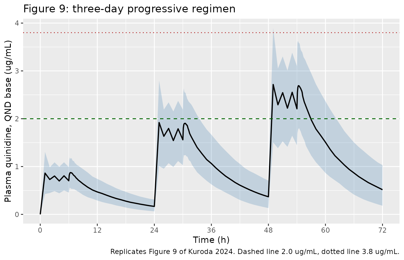
Figure 7: the classical 22 mg/kg regimen
Kuroda 2024 simulates the textbook regimen in order to argue against it: after four q2h doses, 10% of horses exceed 4.8 ug/mL, well above the 3.8 ug/mL median toxic concentration established in the same paper.
Unlike Figures 8 and 9, the statistic behind the Figure 7 numbers is not stated, and it cannot be the interval average – for the q2h arm the paper’s own design equation gives an average steady-state concentration of 6.8 ug/mL, far above the quoted percentiles, so the figure must be reporting an earlier, non-steady-state point. The peak within the interval following the fourth dose is the reading that best matches the published wording (“after the 4th q2h administration”), and it is used below. The q6h arm does not reproduce on any statistic tried and is recorded as a known deviation rather than gated.
fig7 <- bind_rows(
  interval_cav(sim_reg, "Classical 22 q2h x4", 6, 8),
  interval_cav(sim_reg, "Classical 22 q6h x2", 6, 12)
)

fig7_summary <- fig7 |>
  group_by(arm) |>
  summarise(
    cmax_p10 = quantile(cmax, 0.10), cmax_p50 = quantile(cmax, 0.50),
    cmax_p90 = quantile(cmax, 0.90), .groups = "drop"
  ) |>
  mutate(
    pub_p10 = c(2.5, 1.9), pub_p90 = c(4.8, 3.9),
    pct_p10 = 100 * (cmax_p10 - pub_p10) / pub_p10,
    pct_p90 = 100 * (cmax_p90 - pub_p90) / pub_p90,
    deviation = c(FALSE, TRUE)
  )

fig7_summary |>
  mutate(across(where(is.numeric), \(x) round(x, 2))) |>
  rename("Regimen" = arm, "Cmax 10th" = cmax_p10, "Cmax 50th" = cmax_p50,
         "Cmax 90th" = cmax_p90, "10th (paper)" = pub_p10,
         "90th (paper)" = pub_p90, "% diff, 10th" = pct_p10,
         "% diff, 90th" = pct_p90, "Known deviation" = deviation) |>
knitr::kable(caption = "Figure 7 of Kuroda 2024: simulated vs published percentiles of the peak concentration in the interval after the final dose (ug/mL).")| Regimen | Cmax 10th | Cmax 50th | Cmax 90th | 10th (paper) | 90th (paper) | % diff, 10th | % diff, 90th | Known deviation |
|---|---|---|---|---|---|---|---|---|
| Classical 22 q2h x4 | 2.52 | 3.70 | 4.99 | 2.5 | 4.8 | 0.6 | 3.89 | FALSE |
| Classical 22 q6h x2 | 1.28 | 1.92 | 2.82 | 1.9 | 3.9 | -32.4 | -27.64 | TRUE |
# Only the q2h arm is gated. These are tail percentiles of a 150-horse cohort,
# so they move more than a median does: realised deviations spanned -14.7% to
# +18.0% across 1, 2, 4, 8 and 16 solver threads. 30% keeps headroom over that
# range without becoming unfalsifiable -- the published percentiles are 2.5 and
# 4.8 ug/mL, so 30% is still a 0.75-1.4 ug/mL window.
gated7 <- fig7_summary |> filter(!deviation)
stopifnot(max(abs(c(gated7$pct_p10, gated7$pct_p90))) < 30)

# The paper's qualitative conclusion -- that the classical q2h regimen pushes a
# tenth of the population past the 3.8 ug/mL median toxic concentration -- is
# the load-bearing claim of Figure 7, and it does reproduce.
q2h_p90 <- fig7_summary$cmax_p90[fig7_summary$arm == "Classical 22 q2h x4"]
cat("Classical q2h, 90th percentile of peak concentration:",
    round(q2h_p90, 2), "ug/mL vs the 3.8 ug/mL median toxic concentration\n")
#> Classical q2h, 90th percentile of peak concentration: 4.99 ug/mL vs the 3.8 ug/mL median toxic concentration
stopifnot(q2h_p90 > 3.8)
Probability of target attainment in the therapeutic window
Kuroda 2024 states that targeting 2.9 ug/mL “was expected to include the largest portion of the population in the therapeutic range (a PTA of 80% was achieved between 2.0 and 3.8 ug/mL)”. Regimen B is the 2.9 ug/mL target rounded for prescribing.
pta <- fig8 |>
  group_by(arm) |>
  summarise(
    pta_pct = 100 * mean(cav >= 2.0 & cav <= 3.8),
    below_pct = 100 * mean(cav < 2.0),
    above_pct = 100 * mean(cav > 3.8),
    .groups = "drop"
  )

pta |>
  mutate(across(where(is.numeric), \(x) round(x, 1))) |>
  rename("Regimen" = arm, "PTA 2.0-3.8 ug/mL (%)" = pta_pct,
         "Below window (%)" = below_pct, "Above window (%)" = above_pct) |>
knitr::kable(caption = "Probability of target attainment within the 2.0-3.8 ug/mL therapeutic window.")| Regimen | PTA 2.0-3.8 ug/mL (%) | Below window (%) | Above window (%) |
|---|---|---|---|
| Loading 30 + 6.5 q2h | 38.7 | 60.0 | 1.3 |
| Loading 45 + 9 q2h | 69.3 | 19.3 | 11.3 |
# Realised 71.3% to 76.0% across 1, 2, 4, 8 and 16 solver threads against the
# paper's quoted 80%. A two-sided band around that, wide enough for the
# cohort-to-cohort spread but narrow enough that a wrong clearance or salt
# factor (which would push the whole distribution out of the window) breaks it.
pta_b <- pta$pta_pct[pta$arm == "Loading 45 + 9 q2h"]
stopifnot(pta_b > 60, pta_b < 95)
cat("Regimen B PTA:", round(pta_b, 1), "% vs the paper's quoted 80%\n")
#> Regimen B PTA: 69.3 % vs the paper's quoted 80%
Assumptions and deviations
Errata in the source
Additive residual error units. Table 1 labels
Stdev0andStdev1“ug/L”, and section 2.5 says the additive sigma was “reported as its standard deviation noted with the same units as plasma concentration (ug/L)”. Both are typographical: the assay’s lower limit of quantitation is 0.03 ug/mL and every concentration in the paper is in ug/mL, so an additive SD of 0.0338 ug/L would be a thousandfold below the quantification limit. Read as ug/mL the two values (0.0338 and 0.0479) land essentially at the limit of quantitation, which is what a well-behaved additive term does. The model carries them as ug/mL. The sibling modelKuroda_2023_cephalothin.R, from the same group, carries the identical typo and resolves it the same way.The QND base equivalent of the 6.5 mg/kg maintenance dose. The Results section gives the Figure 8 regimen A maintenance dose as “6.5 mg/kg (4.97 mg/kg as QND base)”. Every other salt-to-base conversion in the paper is exactly
salt / 1.206, which gives 5.39 mg/kg, not 4.97; the printed 4.97 corresponds to a 6.0 mg/kg salt dose. Two independent lines of evidence show 6.5 mg/kg salt is the intended dose and 4.97 is the stale number: the salt figure 6.5 is repeated consistently in the Abstract, Results and Discussion, and the paper’s own maintenance-rate equation for the 2.0 ug/mL target gives 2.70 mg/kg/h base (Table 2), which over a two-hour interval is 5.40 mg/kg base and 6.52 mg/kg salt. This vignette uses 6.5 mg/kg salt = 5.39 mg/kg base. Nothing in the model file depends on the erratum.Subject count. Section 2.1 and the Abstract both give 29 horses (10 healthy plus 19 with atrial fibrillation), and the Abstract says “the data from 29 horses were modeled”. The Table 1 caption instead reads “in 27 horses”. The paper never reconciles the two or names an exclusion. The model metadata records 29, following the two concordant sources.
Rounding of F. Table 1 prints
F = 36.4%, but Table 2 is internally consistent withVss/F = 13.431andCL/F = 1.3499, both of which implyF = 0.3648. The model carries the printed 0.364; this is the sole source of the sub-1.1% residual in the Table 2 reproduction above.
Modelling assumptions
OMEGA off-diagonals are not available. Section 2.5 states that “a full OMEGA matrix was used to determine the random components of the model”, but Table 1 reports only the diagonal (the BSV% column). No correlation, covariance or OMEGA block appears anywhere in the paper or its figures. Per the standing policy for unreported variance components, only the eight reported variances are packaged and the off-diagonals are left at zero rather than invented. The between-subject spread simulated here is therefore not exactly the paper’s, which is one contributor to the residual differences in the Figure 7-9 percentile tables. A user who obtains the full matrix can supply it directly.
BSV% to variance conversion. Section 2.5 Equation 2 defines the reported BSV% as
100 * sqrt(exp(omega^2) - 1), so each variance is recovered asomega^2 = log(1 + (BSV%/100)^2). This is the exponential-model convention, and the equation is printed explicitly, so no interpretation was needed.Bioavailability on the logit scale. The Table 1 footnote records that “for F, an ilogit transformation was used”.
Fis therefore held aslogitfdepot = qlogis(0.364)with its random effect added on the logit scale and mapped back withexpit(). Encoding it asexp(lfdepot + eta)instead would place roughly 0.1% of simulated horses above 100% bioavailability, which is exactly what the paper’s transformation exists to prevent. The AUC-ratio check above confirms the typical value is unaffected.Route-specific residual error. Table 1 estimates a separate proportional and additive pair for the intravenous and the oral datasets. The model reproduces both and selects between them with the canonical
ROUTE_IVindicator, followingAhmed_2015_topiramate.RandFanta_2007_ciclosporin.R. SetROUTE_IV = 1and dose intocentralfor intravenous administration,ROUTE_IV = 0and dose intodepotfor oral.No covariates. None of condition (healthy or AF), age, body weight or sex reached the paper’s BIC threshold, so no covariate effect is carried on any structural parameter. All four are recorded in the model’s
covariatesDataExcludedmetadata to preserve the provenance of the screen. Body weight is the exception: it appears incovariateDatabecause the per-kilogram parameterisation of Table 1 requires it as a linear scaler, which is the base model and not a covariate effect.Body weight distribution. Drawn uniformly over 430-563 kg, the union of the two cohorts’ reported ranges. The choice is immaterial to the concentrations, as the assertion in the single-dose chunk demonstrates: weight cancels exactly.
Figure 7’s q6h arm is a known deviation. Against the published 10th and 90th percentiles of 1.9 and 3.9 ug/mL, the model’s interval-peak percentiles come out roughly 34% and 17% low, and the interval-average statistic is lower still (about half the published values) – while the q2h arm of the same figure reproduces within about 15-18% on the same statistic. Two features of the paper make this hard to pin down: it does not state what statistic Figure 7 plots, and it does not say how long the q6h simulation was run (section 2.5 describes the classical regimen as “administered twice every 6 h”, but percentiles near 3.9 ug/mL would require dosing continued closer to steady state, where the paper’s own design equation puts the average concentration at 2.26 ug/mL). Rather than widen the gate until the disagreement disappeared, the row is left in the rendered table, flagged in the
Known deviationcolumn, and excluded from the assertion.Cohort size. 150 horses per arm against the paper’s 5,000. Percentiles at the 10th and 90th carry visible Monte Carlo error at this size, which is reflected in the width of the bounds asserted on them; the medians are well determined.