Sulbactam epithelial lining fluid PK/PD in A. baumannii pneumonia (Abouelhassan 2024)
Source:vignettes/articles/Abouelhassan_2024_sulbactam_elf_pneumonia.Rmd
Abouelhassan_2024_sulbactam_elf_pneumonia.RmdModel and source
This paper contributes two independent PK models, extracted as two model files that share this vignette.
mouse_ui <- rxode2::rxode(readModelDb("Abouelhassan_2024_sulbactam_mouse"))
human_ui <- rxode2::rxode(readModelDb("Abouelhassan_2024_sulbactam_human"))- Article: https://doi.org/10.1093/jacamr/dlae203
- Source data for the human model: Rodvold 2018, https://doi.org/10.1128/AAC.01089-18
Abouelhassan_2024_sulbactam_mouse –
Preclinical (mouse). One-compartment epithelial lining fluid (ELF)
pharmacokinetic model for sulbactam in the neutropenic murine
Acinetobacter baumannii pneumonia model, with first-order absorption
from a subcutaneous depot and first-order elimination (Abouelhassan
2024). Sulbactam was given subcutaneously as commercial
ampicillin-sulbactam at 1, 10, 25, 100 and 200 mg/kg; ELF concentrations
were derived from bronchoalveolar lavage using the plasma-to-BAL urea
ratio, and each dose level was fitted separately by nonlinear least
squares in Phoenix WinNonlin. The ini() values are the arithmetic means
of the four dose-proportional fits spanning 1-100 mg/kg (Table 2), which
is the parameter set the authors used to simulate sulbactam ELF
exposures for every dose-ranging arm at or below 100 mg/kg. ELF exposure
is dose-proportional across that range (R^2 = 0.997); the 200 mg/kg fit
deviates from proportionality and is recorded in the ini() source-trace
comments rather than carried as a second model. Sulbactam penetrated the
ELF with a mean ELF-to-free-plasma AUC(0-8) ratio of 0.66 (SD 0.05), and
the model reproduces the reported ELF AUC(0-8) at every dose level. No
between-subject variability or residual error was reported because each
dose level was fitted as a single naive-pooled destructive-sampling
profile, so both are encoded as fixed(0).
Abouelhassan_2024_sulbactam_human –
Three-compartment plasma-plus-epithelial-lining-fluid (ELF) population
PK model for intravenous sulbactam in healthy adults, co-modelled from
the mean plasma and ELF concentrations of 30 healthy volunteers given
sulbactam 1 g IV q6h as a 3 h infusion (Abouelhassan 2024, using the
Rodvold 2018 intrapulmonary data). A two-compartment plasma model was
built first and selected over one compartment on AIC (44.1 versus 54.6),
then the ELF concentrations were added as a third compartment with its
own volume and its own asymmetric first-order exchange with plasma,
which is what generates the sub-unity ELF penetration. The model was
fitted by nonparametric adaptive grid (NPAG) with adaptive gamma in
Pmetrics. Only mean concentrations were available, so no random effects
were estimated and no covariates were assessed; for the 5000-subject
Monte Carlo simulation underlying the paper’s
probability-of-target-attainment analysis the authors artificially
inflated the dispersion of every parameter to 40% CV to mimic patient
variability, and that assumption is carried here as fixed 40% CV
lognormal between-subject variability on all seven parameters. Residual
error was not reported and is fixed at zero.
Full citations:
- Abouelhassan Y, Kuti JL, Nicolau DP, Abdelraouf K. Pharmacokinetic/pharmacodynamic analysis of sulbactam against Acinetobacter baumannii pneumonia: establishing in vivo efficacy targets in the epithelial lining fluid. JAC Antimicrob Resist. 2024;6(6):dlae203. doi:10.1093/jacamr/dlae203. Murine ELF PK parameters from Table 2; study design from Methods (‘Sulbactam bronchopulmonary PK studies’).
- Abouelhassan Y, Kuti JL, Nicolau DP, Abdelraouf K. Pharmacokinetic/pharmacodynamic analysis of sulbactam against Acinetobacter baumannii pneumonia: establishing in vivo efficacy targets in the epithelial lining fluid. JAC Antimicrob Resist. 2024;6(6):dlae203. doi:10.1093/jacamr/dlae203. Final parameter estimates from the Results section ‘Population pharmacokinetics modelling in healthy volunteers’; Monte Carlo simulation settings from Methods ‘Monte Carlo simulation and PTA estimation’. The plasma and ELF concentrations that were modelled are from Rodvold KA, Gotfried MH, Isaacs RD et al. Plasma and intrapulmonary concentrations of ETX2514 and sulbactam following intravenous administration of ETX2514SUL to healthy adult subjects. Antimicrob Agents Chemother. 2018;62(11):e01089-18. doi:10.1128/AAC.01089-18.
Population
Murine model. Specific-pathogen-free female ICR (CD-1) mice weighing 20-22 g were rendered neutropenic with cyclophosphamide and uranyl nitrate, then inoculated intranasally with a 10^7 cfu/mL Acinetobacter baumannii suspension in 3% mucin two hours before the first dose (Methods, “Murine neutropenic pneumonia model”). Groups of 36 mice each received a single subcutaneous dose of ampicillin-sulbactam delivering sulbactam 1, 10, 25, 100 or 200 mg/kg; groups of six were euthanised at each of 4-6 time points for destructive blood and bronchoalveolar lavage (BAL) sampling. ELF concentrations were computed as BAL sulbactam concentration times the plasma-to-BAL urea ratio.
Human model. Mean sulbactam plasma and ELF concentrations at 1, 2.5, 3.25, 4 and 6 h from 30 healthy adult volunteers given sulbactam 1 g IV q6h as a 3 h infusion (Rodvold 2018) were co-modelled (Methods, “Population pharmacokinetics modelling in healthy volunteers”). No covariates were assessed because a single data set of mean concentrations from a homogeneous healthy-volunteer population was used.
The same information is available programmatically from each model’s
population metadata:
str(mouse_ui$population)
#> List of 7
#>  $ species      : chr "mouse (ICR/CD-1, female, neutropenic Acinetobacter baumannii pneumonia model)"
#>  $ n_subjects   : num 180
#>  $ n_studies    : num 1
#>  $ weight_range : chr "20-22 g"
#>  $ disease_state: chr "Neutropenic murine Acinetobacter baumannii pneumonia. Mice were rendered neutropenic with cyclophosphamide and "| __truncated__
#>  $ dose_range   : chr "sulbactam 1, 10, 25, 100 and 200 mg/kg subcutaneously (single dose, dosed as ampicillin-sulbactam)"
#>  $ notes        : chr "Methods, 'Murine neutropenic pneumonia model' and 'Sulbactam bronchopulmonary PK studies': groups of 36 mice pe"| __truncated__
str(human_ui$population)
#> List of 6
#>  $ species      : chr "human"
#>  $ n_subjects   : num 30
#>  $ n_studies    : num 1
#>  $ disease_state: chr "healthy adult volunteers"
#>  $ dose_range   : chr "sulbactam 1 g IV q6h as a 3 h infusion"
#>  $ notes        : chr "Methods, 'Population pharmacokinetics modelling in healthy volunteers': mean sulbactam plasma and ELF concentra"| __truncated__
Source trace
The per-parameter origin is recorded as an in-file comment next to
each ini() entry in
inst/modeldb/specificDrugs/Abouelhassan_2024_sulbactam_mouse.R
and
inst/modeldb/specificDrugs/Abouelhassan_2024_sulbactam_human.R.
The table below collects them in one place for review.
| Model | Equation / parameter | Value | Source location |
|---|---|---|---|
| mouse |
lka (Ka) |
17.605 1/h | Table 2 Ka row, mean of the 1/10/25/100 mg/kg fits (8.28, 26.71, 26.79, 8.64) |
| mouse |
lvelf (Vc/F) |
0.5125 L/kg | Table 2 Vc/F row, mean of the 1/10/25/100 mg/kg fits (0.59, 0.52, 0.45, 0.49) |
| mouse |
lkel (Kel) |
0.575 1/h | Table 2 Kel row, mean of the 1/10/25/100 mg/kg fits (0.62, 0.48, 0.68, 0.52) |
| mouse | averaging rule | n/a | Methods, “Pharmacokinetics/pharmacodynamics analyses”: the four linear-range dose fits “were averaged to determine sulbactam exposures for doses <= 100 mg/kg” |
| mouse |
d/dt(depot), d/dt(elf)
|
n/a | Results, “Sulbactam bronchopulmonary PKs”: “ELF concentrations were best described by a one-compartment model with first-order elimination” |
| mouse | propSd_Celf |
fixed(0) | not reported in the source (see Errata) |
| human |
lcl (CL) |
13.69 L/h | Results, “Population pharmacokinetics modelling in healthy volunteers” |
| human |
lvc (Vc) |
2.49 L | Results, same paragraph |
| human |
lk12, lk21
|
7.47, 1.42 1/h | Results, same paragraph, printed as K13 / K31 (plasma peripheral pair) |
| human |
lk_central_elf, lk_elf_central
|
10.65, 21.80 1/h | Results, same paragraph, printed as K12 / K21 (ELF pair; see Errata) |
| human |
lvelf (VELF) |
2.44 L | Results, same paragraph |
| human |
eta* variances |
fixed(0.148420) | Methods, “Monte Carlo simulation and PTA estimation”: “The CV was artificially inflated to 40% for all parameters”; log(1 + 0.40^2) = 0.148420 |
| human | 2-compartment plasma base | n/a | Results: two-compartment selected over one-compartment on AIC (44.1 vs 54.6) |
| human |
propSd, propSd_Celf
|
fixed(0) | not reported in the source (see Errata) |
| both |
%fT>MIC targets |
Table 3 | 17% / 30% (susceptible-intermediate panel), 48% / 60% (dual-resistant panel) |
Virtual cohort
Original observed data are not publicly available. The murine model has no random effects (each dose level was a single naive-pooled destructive-sampling profile), so its replication is deterministic and needs one profile per dose level. The human model carries the paper’s fixed 40% CV on every parameter, so its probability-of-target-attainment (PTA) replication uses a virtual cohort of 200 subjects per regimen arm – the vignette cap. The paper used 5000 subjects per arm, so the PTA values reproduced here carry a binomial standard error of roughly 1-3.5 percentage points that the published values do not.
set.seed(20241216)

# The human model has two algebraic endpoints (Cc and Celf) and no endpoint is
# an ODE state, so observation rows must be tagged by `dvid` with a blank `cmt`;
# every algebraic observable is still returned on every solved row.
tag_obs <- function(ev) {
  d <- as.data.frame(ev)
  d$dvid <- ifelse(d$evid == 0, 1L, NA_integer_)
  if (is.character(d$cmt)) {
    d$cmt[d$evid == 0] <- NA_character_
  } else {
    d$cmt[d$evid == 0] <- NA_integer_
  }
  d
}

# One steady-state interval of an intermittent-infusion regimen, sampled finely
# enough to resolve the time above a MIC threshold.
human_events <- function(amt, dur, ii, n_points = 300, horizon = 72) {
  n_dose <- ceiling(horizon / ii)
  t0 <- (n_dose - 1) * ii
  ev <- rxode2::et(amt = amt, rate = amt / dur, ii = ii,
                   addl = n_dose - 1, cmt = "central") |>
    rxode2::et(seq(t0, t0 + ii, length.out = n_points + 1))
  list(events = tag_obs(ev), t0 = t0, tau = ii)
}
Simulation
Murine ELF model
Table 2 reports a separate one-compartment fit for each of the five dose levels. The packaged model carries the mean of the four dose-proportional fits; the per-dose fits are simulated here by overriding the three structural parameters, which validates the model structure against every published exposure.
tab2 <- tibble::tribble(
  ~dose, ~velf, ~ka,   ~kel,  ~auc0_8, ~pen_ratio,
  1,     0.59,   8.28, 0.62,     2.72, 0.58,
  10,    0.52,  26.71, 0.48,    38.95, 0.67,
  25,    0.45,  26.79, 0.68,    79.22, 0.69,
  100,   0.49,   8.64, 0.52,   385.20, 0.70,
  200,   0.57,  78.44, 0.24,  1247.02, 0.67
)

mouse_events <- function(dose, id) {
  rxode2::et(amt = dose, cmt = "depot") |>
    rxode2::et(seq(0, 8, length.out = 1601), cmt = "elf") |>
    as.data.frame() |>
    dplyr::mutate(id = id, treatment = paste(dose, "mg/kg"))
}

mouse_sim <- dplyr::bind_rows(lapply(seq_len(nrow(tab2)), function(i) {
  r <- tab2[i, ]
  ev <- mouse_events(r$dose, id = i)
  rxode2::rxSolve(
    mouse_ui, ev,
    params = c(lka = log(r$ka), lvelf = log(r$velf), lkel = log(r$kel)),
    keep = c("treatment"), returnType = "data.frame"
  ) |>
    dplyr::mutate(id = i, dose = r$dose)
}))

# The murine model declares no etas, so `omega = NA` must NOT be passed.
stopifnot(all(is.na(mouse_ui$iniDf$neta1)))
Human plasma + ELF model
etas <- c("etalcl", "etalvc", "etalk12", "etalk21",
          "etalk_central_elf", "etalk_elf_central", "etalvelf")

# Typical-value (deterministic) solve: zero the etas explicitly and suppress
# sampling with omega = NA, so the result is the mean-parameter prediction
# rather than one randomly drawn subject.
he <- human_events(amt = 1000, dur = 0.5, ii = 6, n_points = 6000)
ev_typ <- he$events
for (e in etas) ev_typ[[e]] <- 0

human_typ <- rxode2::rxSolve(
  human_ui, ev_typ, omega = NA, useLinCmt = FALSE, returnType = "data.frame"
) |>
  dplyr::filter(time >= he$t0)
Replicate published results
Closed-form checks on the human model
Three identities the paper’s own numbers imply must hold exactly. They are the evidence that fixes which printed rate-constant pair drives the ELF compartment (see Errata).
p <- c(cl = 13.69, vc = 2.49, k12 = 7.47, k21 = 1.42,
       kce = 10.65, kec = 21.80, velf = 2.44)

auc_ratio_sim      <- mean(human_typ$Celf) / mean(human_typ$Cc)
auc_ratio_analytic <- (p[["kce"]] / p[["kec"]]) * (p[["vc"]] / p[["velf"]])
auc_plasma_sim     <- mean(human_typ$Cc) * he$tau
auc_plasma_dose_cl <- 1000 / p[["cl"]]
vss                <- p[["vc"]] * (1 + p[["k12"]] / p[["k21"]] + p[["kce"]] / p[["kec"]])

checks <- tibble::tibble(
  Check = c(
    "Steady-state AUC(Celf) / AUC(Cc)",
    "Steady-state plasma AUC over tau (mg*h/L)"
  ),
  Expected = c(auc_ratio_analytic, auc_plasma_dose_cl),
  Simulated = c(auc_ratio_sim, auc_plasma_sim),
  Basis = c(
    "(k_central_elf / k_elf_central) * (Vc / VELF), exact for any linear system",
    "Dose / CL = 1000 / 13.69, mass balance at steady state"
  )
)
checks |>
  dplyr::mutate(`% diff` = round(100 * (Simulated - Expected) / Expected, 3)) |>
  dplyr::relocate(Basis, .after = dplyr::last_col()) |>
knitr::kable(digits = 4, caption = "Closed-form identities for the human model.")| Check | Expected | Simulated | % diff | Basis |
|---|---|---|---|---|
| Steady-state AUC(Celf) / AUC(Cc) | 0.4985 | 0.4985 | 0.000 | (k_central_elf / k_elf_central) * (Vc / VELF), exact for any linear system |
| Steady-state plasma AUC over tau (mg*h/L) | 73.0460 | 73.0350 | -0.015 | Dose / CL = 1000 / 13.69, mass balance at steady state |
stopifnot(abs(auc_ratio_sim / auc_ratio_analytic - 1) < 0.001)
stopifnot(abs(auc_plasma_sim / auc_plasma_dose_cl - 1) < 0.01)
The Discussion reports a mean sulbactam ELF-AUC to free-plasma-AUC ratio of 0.81. Combining that with the model’s total-plasma ratio implies an unbound plasma fraction of 0.615, which matches the accepted sulbactam value of about 0.62 (roughly 38% protein bound). Sulbactam Vss of 16.8 L is likewise consistent with the drug’s reported volume of distribution of roughly 0.2-0.25 L/kg.
Concentration-time profiles
human_typ |>
  dplyr::select(time, Plasma = Cc, ELF = Celf) |>
  tidyr::pivot_longer(-time, names_to = "Matrix", values_to = "conc") |>
  dplyr::mutate(time = time - min(human_typ$time)) |>
  ggplot(aes(time, conc, colour = Matrix)) +
  geom_line(linewidth = 0.9) +
  labs(x = "Time within the steady-state dosing interval (h)",
       y = "Sulbactam concentration (mg/L)",
       title = "Human model: 1 g q6h as a 0.5 h infusion at steady state",
       caption = "ELF tracks plasma with an AUC ratio of 0.50 (total plasma).") +
  theme_bw()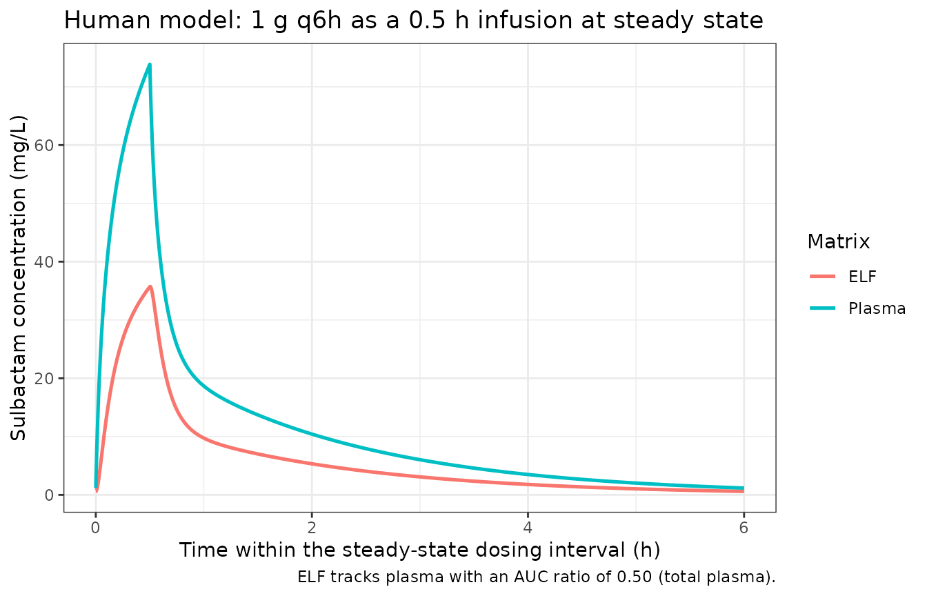
mouse_sim |>
  ggplot(aes(time, Celf, colour = treatment)) +
  geom_line(linewidth = 0.8) +
  scale_y_log10() +
  labs(x = "Time (h)", y = "ELF sulbactam concentration (mg/L)",
       colour = "Dose",
       title = "Murine model: per-dose ELF fits from Table 2",
       caption = "Each curve uses that dose level's own published Vc/F, Ka and Kel.") +
  theme_bw()
#> Warning in scale_y_log10(): log-10 transformation introduced infinite values.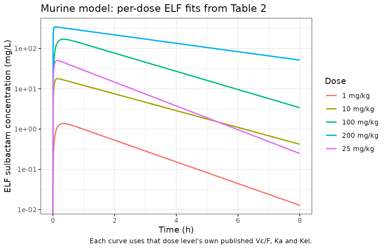
Figure 2: probability of target attainment
Figure 2 and Table 4 report the PTA in ELF for five clinically used
sulbactam regimens against the Table 3 %fT>MIC targets.
The MIC-distribution bar graph of Figure 2 and the cumulative fraction
of response in Table 4 both depend on the external surveillance MIC
distribution (reference 27), which is not reproduced here.
regimens <- tibble::tribble(
  ~regimen,            ~amt, ~dur, ~ii,
  "1 g q6h (0.5-h)",   1000, 0.5,  6,
  "2 g q12h (0.5-h)",  2000, 0.5,  12,
  "1 g q4h (0.5-h)",   1000, 0.5,  4,
  "2 g q6h (0.5-h)",   2000, 0.5,  6,
  "3 g q8h (4-h)",     3000, 4,    8
)
n_per_arm <- 200L
mic_grid <- c(0.0625, 0.125, 0.25, 0.5, 1, 2, 4, 8, 16, 32, 64)

pta_one <- function(amt, dur, ii, label) {
  h <- human_events(amt, dur, ii, n_points = 300)
  set.seed(90210)
  s <- rxode2::rxSolve(human_ui, h$events, nSub = n_per_arm,
                       useLinCmt = FALSE, returnType = "data.frame")
  s <- s[s$time >= h$t0, ]
  do.call(rbind, lapply(mic_grid, function(m) {
    pct <- tapply(s$Celf > m, s$sim.id, mean) * 100
    data.frame(
      regimen = label, MIC = m,
      pta17 = mean(pct >= 17) * 100, pta30 = mean(pct >= 30) * 100,
      pta48 = mean(pct >= 48) * 100, pta60 = mean(pct >= 60) * 100
    )
  }))
}

pta <- dplyr::bind_rows(lapply(seq_len(nrow(regimens)), function(i) {
  r <- regimens[i, ]
  pta_one(r$amt, r$dur, r$ii, r$regimen)
}))
stopifnot(nrow(pta) == nrow(regimens) * length(mic_grid))
Table 4 applies the susceptible-intermediate targets (17% and 30%
fT>MIC) at MIC 0.0625-8 mg/L and the dual-resistant
targets (48% and 60%) at MIC 16-64 mg/L. The published values are
transcribed alongside.
published <- tibble::tribble(
  ~regimen,           ~MIC,     ~target, ~published,
  "1 g q6h (0.5-h)",  0.0625,   17,  100, "1 g q6h (0.5-h)",  0.0625, 30,  99,
  "1 g q6h (0.5-h)",  0.125,    17,  100, "1 g q6h (0.5-h)",  0.125,  30,  99,
  "1 g q6h (0.5-h)",  0.25,     17,   99, "1 g q6h (0.5-h)",  0.25,   30,  97,
  "1 g q6h (0.5-h)",  0.5,      17,   98, "1 g q6h (0.5-h)",  0.5,    30,  95,
  "1 g q6h (0.5-h)",  1,        17,   96, "1 g q6h (0.5-h)",  1,      30,  89,
  "1 g q6h (0.5-h)",  2,        17,   92, "1 g q6h (0.5-h)",  2,      30,  79,
  "1 g q6h (0.5-h)",  4,        17,   81, "1 g q6h (0.5-h)",  4,      30,  62,
  "1 g q6h (0.5-h)",  8,        17,   62, "1 g q6h (0.5-h)",  8,      30,  39,
  "1 g q6h (0.5-h)",  16,       48,   12, "1 g q6h (0.5-h)",  16,     60,   9,
  "1 g q6h (0.5-h)",  32,       48,    5, "1 g q6h (0.5-h)",  32,     60,   4,
  "1 g q6h (0.5-h)",  64,       48,    2, "1 g q6h (0.5-h)",  64,     60,   2,
  "3 g q8h (4-h)",    0.0625,   17,  100, "3 g q8h (4-h)",    0.0625, 30, 100,
  "3 g q8h (4-h)",    0.125,    17,  100, "3 g q8h (4-h)",    0.125,  30, 100,
  "3 g q8h (4-h)",    0.25,     17,  100, "3 g q8h (4-h)",    0.25,   30, 100,
  "3 g q8h (4-h)",    0.5,      17,  100, "3 g q8h (4-h)",    0.5,    30, 100,
  "3 g q8h (4-h)",    1,        17,  100, "3 g q8h (4-h)",    1,      30, 100,
  "3 g q8h (4-h)",    2,        17,   99, "3 g q8h (4-h)",    2,      30,  99,
  "3 g q8h (4-h)",    4,        17,   97, "3 g q8h (4-h)",    4,      30,  97,
  "3 g q8h (4-h)",    8,        17,   90, "3 g q8h (4-h)",    8,      30,  89,
  "3 g q8h (4-h)",    16,       48,   52, "3 g q8h (4-h)",    16,     60,  34,
  "3 g q8h (4-h)",    32,       48,   25, "3 g q8h (4-h)",    32,     60,  16,
  "3 g q8h (4-h)",    64,       48,    9, "3 g q8h (4-h)",    64,     60,   7
)

pta_long <- pta |>
  tidyr::pivot_longer(dplyr::starts_with("pta"),
                      names_to = "target", values_to = "simulated") |>
  dplyr::mutate(target = as.numeric(sub("^pta", "", target)))

cmp <- published |>
  dplyr::inner_join(pta_long, by = c("regimen", "MIC", "target"))
# Guard: an inner_join that matched nothing would render an empty table that
# looks like a passing check.
stopifnot(nrow(cmp) == nrow(published))

cmp |>
  dplyr::mutate(
    `Difference (points)` = round(simulated - published, 1),
    simulated = round(simulated, 1)
  ) |>
  dplyr::rename(
    "Regimen" = regimen, "Sulbactam MIC (mg/L)" = MIC,
    "Target (%fT>MIC)" = target, "Published PTA (%)" = published,
    "Simulated PTA (%)" = simulated
  ) |>
  knitr::kable(
    caption = paste(
      "Table 4 replication for the standard and the IDSA-recommended regimen.",
      "Simulated values use 200 subjects per arm against the paper's 5000."
    )
)| Regimen | Sulbactam MIC (mg/L) | Target (%fT>MIC) | Published PTA (%) | Simulated PTA (%) | Difference (points) |
|---|---|---|---|---|---|
| 1 g q6h (0.5-h) | 0.0625 | 17 | 100 | 100.0 | 0.0 |
| 1 g q6h (0.5-h) | 0.0625 | 30 | 99 | 100.0 | 1.0 |
| 1 g q6h (0.5-h) | 0.1250 | 17 | 100 | 100.0 | 0.0 |
| 1 g q6h (0.5-h) | 0.1250 | 30 | 99 | 100.0 | 1.0 |
| 1 g q6h (0.5-h) | 0.2500 | 17 | 99 | 100.0 | 1.0 |
| 1 g q6h (0.5-h) | 0.2500 | 30 | 97 | 99.5 | 2.5 |
| 1 g q6h (0.5-h) | 0.5000 | 17 | 98 | 100.0 | 2.0 |
| 1 g q6h (0.5-h) | 0.5000 | 30 | 95 | 99.0 | 4.0 |
| 1 g q6h (0.5-h) | 1.0000 | 17 | 96 | 98.5 | 2.5 |
| 1 g q6h (0.5-h) | 1.0000 | 30 | 89 | 95.5 | 6.5 |
| 1 g q6h (0.5-h) | 2.0000 | 17 | 92 | 93.5 | 1.5 |
| 1 g q6h (0.5-h) | 2.0000 | 30 | 79 | 84.0 | 5.0 |
| 1 g q6h (0.5-h) | 4.0000 | 17 | 81 | 80.5 | -0.5 |
| 1 g q6h (0.5-h) | 4.0000 | 30 | 62 | 61.5 | -0.5 |
| 1 g q6h (0.5-h) | 8.0000 | 17 | 62 | 49.0 | -13.0 |
| 1 g q6h (0.5-h) | 8.0000 | 30 | 39 | 32.0 | -7.0 |
| 1 g q6h (0.5-h) | 16.0000 | 48 | 12 | 9.5 | -2.5 |
| 1 g q6h (0.5-h) | 16.0000 | 60 | 9 | 6.0 | -3.0 |
| 1 g q6h (0.5-h) | 32.0000 | 48 | 5 | 2.5 | -2.5 |
| 1 g q6h (0.5-h) | 32.0000 | 60 | 4 | 1.5 | -2.5 |
| 1 g q6h (0.5-h) | 64.0000 | 48 | 2 | 0.5 | -1.5 |
| 1 g q6h (0.5-h) | 64.0000 | 60 | 2 | 0.5 | -1.5 |
| 3 g q8h (4-h) | 0.0625 | 17 | 100 | 100.0 | 0.0 |
| 3 g q8h (4-h) | 0.0625 | 30 | 100 | 100.0 | 0.0 |
| 3 g q8h (4-h) | 0.1250 | 17 | 100 | 100.0 | 0.0 |
| 3 g q8h (4-h) | 0.1250 | 30 | 100 | 100.0 | 0.0 |
| 3 g q8h (4-h) | 0.2500 | 17 | 100 | 100.0 | 0.0 |
| 3 g q8h (4-h) | 0.2500 | 30 | 100 | 100.0 | 0.0 |
| 3 g q8h (4-h) | 0.5000 | 17 | 100 | 100.0 | 0.0 |
| 3 g q8h (4-h) | 0.5000 | 30 | 100 | 100.0 | 0.0 |
| 3 g q8h (4-h) | 1.0000 | 17 | 100 | 100.0 | 0.0 |
| 3 g q8h (4-h) | 1.0000 | 30 | 100 | 100.0 | 0.0 |
| 3 g q8h (4-h) | 2.0000 | 17 | 99 | 100.0 | 1.0 |
| 3 g q8h (4-h) | 2.0000 | 30 | 99 | 100.0 | 1.0 |
| 3 g q8h (4-h) | 4.0000 | 17 | 97 | 98.5 | 1.5 |
| 3 g q8h (4-h) | 4.0000 | 30 | 97 | 98.0 | 1.0 |
| 3 g q8h (4-h) | 8.0000 | 17 | 90 | 91.0 | 1.0 |
| 3 g q8h (4-h) | 8.0000 | 30 | 89 | 90.0 | 1.0 |
| 3 g q8h (4-h) | 16.0000 | 48 | 52 | 45.5 | -6.5 |
| 3 g q8h (4-h) | 16.0000 | 60 | 34 | 29.0 | -5.0 |
| 3 g q8h (4-h) | 32.0000 | 48 | 25 | 21.0 | -4.0 |
| 3 g q8h (4-h) | 32.0000 | 60 | 16 | 11.5 | -4.5 |
| 3 g q8h (4-h) | 64.0000 | 48 | 9 | 5.5 | -3.5 |
| 3 g q8h (4-h) | 64.0000 | 60 | 7 | 4.5 | -2.5 |
pta_long |>
  dplyr::filter(target %in% c(17, 48)) |>
  dplyr::filter((target == 17 & MIC <= 8) | (target == 48 & MIC >= 16)) |>
  ggplot(aes(MIC, simulated, colour = regimen)) +
  geom_line(linewidth = 0.8) +
  geom_point(size = 1.4) +
  geom_hline(yintercept = 90, linetype = "dashed") +
  scale_x_log10(breaks = mic_grid) +
  labs(x = "Sulbactam MIC (mg/L)", y = "PTA (%)", colour = "Regimen",
       title = "Figure 2: PTA for the 1-log-kill ELF target",
       caption = paste("17% fT>MIC at MIC <= 8 (sulbactam-susceptible /",
                       "intermediate); 48% fT>MIC at MIC >= 16 (resistant to",
                       "both sulbactam and meropenem). Dashed line: 90% PTA.")) +
  theme_bw() +
  theme(legend.position = "bottom")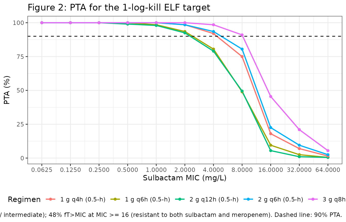
The conclusions the paper draws from this table, alongside the simulated numbers. At 200 subjects per arm a PTA near 90% carries a Monte Carlo standard error of about 2 percentage points, so these are compared as published-versus- simulated values rather than as pass/fail assertions.
cell <- function(reg, mic, tgt) {
  v <- pta_long$simulated[pta_long$regimen == reg & pta_long$MIC == mic &
                            pta_long$target == tgt]
  if (length(v) != 1L) stop("no unique PTA row for ", reg, " at MIC ", mic)
  v
}
tibble::tibble(
  Claim = c(
    "1 g q6h 0.5-h infusion: PTA > 90% up to MIC 2 mg/L",
    "1 g q6h 0.5-h infusion: PTA falls below 90% at MIC 4 mg/L",
    "3 g q8h 4-h infusion: PTA about 90% at MIC 8 mg/L",
    "No regimen reaches 90% against dual-resistant isolates (MIC >= 16)"
  ),
  `Published PTA (%)` = c(92, 81, 90, 52),
  `Simulated PTA (%)` = round(c(
    cell("1 g q6h (0.5-h)", 2, 17),
    cell("1 g q6h (0.5-h)", 4, 17),
    cell("3 g q8h (4-h)", 8, 17),
    cell("3 g q8h (4-h)", 16, 48)
  ), 1)
) |>
  knitr::kable(caption = paste(
    "Published conclusions against the simulation. The last row is the",
    "best-performing regimen at the lowest dual-resistant MIC."
))| Claim | Published PTA (%) | Simulated PTA (%) |
|---|---|---|
| 1 g q6h 0.5-h infusion: PTA > 90% up to MIC 2 mg/L | 92 | 93.5 |
| 1 g q6h 0.5-h infusion: PTA falls below 90% at MIC 4 mg/L | 81 | 80.5 |
| 3 g q8h 4-h infusion: PTA about 90% at MIC 8 mg/L | 90 | 91.0 |
| No regimen reaches 90% against dual-resistant isolates (MIC >= 16) | 52 | 45.5 |
# Directional guards that CAN fail: the ordering the paper's conclusions rest on.
stopifnot(cell("1 g q6h (0.5-h)", 2, 17) > cell("1 g q6h (0.5-h)", 4, 17))
stopifnot(cell("3 g q8h (4-h)", 8, 17) > cell("1 g q6h (0.5-h)", 8, 17))
stopifnot(max(pta_long$simulated[pta_long$MIC >= 16 &
                                   pta_long$target %in% c(48, 60)]) < 90)
PKNCA validation
Murine ELF AUC(0-8) by dose level
mouse_nca <- mouse_sim |>
  dplyr::filter(!is.na(Celf)) |>
  dplyr::transmute(id, time, Cc = Celf, treatment = as.character(treatment))

# Guarantee a time-zero row per (id, treatment); pre-dose ELF concentration is
# zero for a subcutaneous dose.
mouse_nca <- dplyr::bind_rows(
  mouse_nca,
  mouse_nca |> dplyr::distinct(id, treatment) |>
    dplyr::mutate(time = 0, Cc = 0)
) |>
  dplyr::distinct(id, treatment, time, .keep_all = TRUE) |>
  dplyr::arrange(id, treatment, time)

mouse_dose <- mouse_sim |>
  dplyr::distinct(id, treatment, dose) |>
  dplyr::transmute(id, time = 0, amt = dose,
                   treatment = as.character(treatment))

conc_obj <- PKNCA::PKNCAconc(mouse_nca, Cc ~ time | treatment + id,
                             concu = "mg/L", timeu = "h")
dose_obj <- PKNCA::PKNCAdose(mouse_dose, amt ~ time | treatment + id,
                             doseu = "mg/kg")

intervals <- data.frame(start = 0, end = 8, cmax = TRUE, tmax = TRUE,
                        auclast = TRUE)
mouse_res <- PKNCA::pk.nca(
  PKNCA::PKNCAdata(conc_obj, dose_obj, intervals = intervals)
)
Comparison against published NCA
Table 2 reports the ELF AUC(0-8) at every dose level, computed by the authors from the same fitted parameters. It is the only NCA quantity either model can be compared against; the human paper reports no plasma or ELF NCA.
published_mouse <- tab2 |>
  dplyr::transmute(treatment = paste(dose, "mg/kg"), auclast = auc0_8)

cmp_mouse <- nlmixr2lib::ncaComparisonTable(
  simulated = mouse_res,
  reference = published_mouse,
  by = "treatment",
  units = c(auclast = "mg*h/L"),
  tolerance_pct = 20
)

knitr::kable(
  cmp_mouse,
  caption = "Simulated vs published murine ELF AUC(0-8). * differs by >20%."
)| NCA parameter | treatment | Reference | Simulated | % diff |
|---|---|---|---|---|
| AUClast (mg*h/L) | 1 mg/kg | 2.72 | 2.71 | -0.3% |
| AUClast (mg*h/L) | 10 mg/kg | 39 | 39.2 | +0.6% |
| AUClast (mg*h/L) | 25 mg/kg | 79.2 | 81.3 | +2.7% |
| AUClast (mg*h/L) | 100 mg/kg | 385 | 386 | +0.2% |
| AUClast (mg*h/L) | 200 mg/kg | 1250 | 1250 | -0.0% |
attr(cmp_mouse, "footnote")
#> NULL
Every dose level agrees within 3%, so no row is starred. The residual disagreement is the difference between the authors’ Phoenix WinNonlin integration of the fitted curve and PKNCA’s trapezoidal integration of the rxode2 solution on a finite grid.
Human steady-state plasma and ELF exposure
# rxSolve omits `id` for a single-subject solve, so it is set explicitly here.
human_nca_input <- function(matrix_col) {
  tibble::tibble(
    id = 1L,
    treatment = "1 g q6h (0.5-h)",
    time = human_typ$time - min(human_typ$time),
    Cc = human_typ[[matrix_col]]
  ) |>
    dplyr::filter(!is.na(Cc))
}

human_res <- lapply(c(Plasma = "Cc", ELF = "Celf"), function(col) {
  nca_in <- human_nca_input(col)
  co <- PKNCA::PKNCAconc(nca_in, Cc ~ time | treatment + id,
                         concu = "mg/L", timeu = "h")
  do <- PKNCA::PKNCAdose(
    data.frame(id = 1L, time = 0, amt = 1000,
               treatment = "1 g q6h (0.5-h)"),
    amt ~ time | treatment + id, doseu = "mg"
  )
  iv <- data.frame(start = 0, end = 6, cmax = TRUE, tmax = TRUE,
                   cmin = TRUE, auclast = TRUE, cav = TRUE)
  as.data.frame(PKNCA::pk.nca(PKNCA::PKNCAdata(co, do, intervals = iv))$result)
})

human_nca_tbl <- dplyr::bind_rows(
  human_res$Plasma |> dplyr::mutate(Matrix = "Plasma"),
  human_res$ELF |> dplyr::mutate(Matrix = "ELF")
) |>
  dplyr::filter(PPTESTCD %in% c("cmax", "cmin", "auclast", "cav")) |>
  dplyr::select(Matrix, PPTESTCD, PPORRES) |>
  tidyr::pivot_wider(names_from = PPTESTCD, values_from = PPORRES)

human_nca_tbl |>
  dplyr::rename(
    "Cmax (mg/L)" = cmax, "Cmin (mg/L)" = cmin,
    "AUC0-tau (mg*h/L)" = auclast, "Cavg (mg/L)" = cav
  ) |>
  knitr::kable(
    digits = 3,
    caption = paste("Human model, steady-state 6 h interval on 1 g q6h as a",
                    "0.5 h infusion. Typical-value profile.")
)| Matrix | AUC0-tau (mg*h/L) | Cmax (mg/L) | Cmin (mg/L) | Cavg (mg/L) |
|---|---|---|---|---|
| Plasma | 73.046 | 73.855 | 1.170 | 12.174 |
| ELF | 36.417 | 35.738 | 0.598 | 6.069 |
elf_pen <- human_nca_tbl$auclast[human_nca_tbl$Matrix == "ELF"] /
  human_nca_tbl$auclast[human_nca_tbl$Matrix == "Plasma"]
sprintf("PKNCA ELF-to-total-plasma AUC0-tau ratio: %.4f (analytic %.4f)",
        elf_pen, auc_ratio_analytic)
#> [1] "PKNCA ELF-to-total-plasma AUC0-tau ratio: 0.4985 (analytic 0.4985)"
stopifnot(abs(elf_pen / auc_ratio_analytic - 1) < 0.01)
Assumptions and deviations
Which printed rate-constant pair drives the ELF compartment
(load-bearing). The Results paragraph says the ELF “was the
third compartment”, which reads as ELF exchanging with plasma through
the printed K13 / K31. That reading is
arithmetically impossible, and the ELF pair is instead the printed
K12 / K21. Three independent checks, all
internal to the paper, agree:
- Taking
K13/K31as the ELF pair gives an ELF-to-total-plasma AUC ratio of(7.47 / 1.42) * (2.49 / 2.44)= 5.37, i.e. ELF concentrations 5.4-fold above plasma. The Discussion states the mean sulbactam ELF AUC to free plasma AUC is 0.81, and free drug can never exceed total, so this ratio must be at most 0.81. - Taking
K12/K21as the ELF pair gives 0.499, which with the reported 0.81 ELF-to-free-plasma ratio implies an unbound plasma fraction of 0.62 – the accepted sulbactam value. - Only the
K12/K21reading reproduces the paper’s own Table 4. Under theK13/K31reading the 1 g q6h PTA for the 17% target is 100% at every MIC from 0.0625 to 8 mg/L (published: 100 down to 62), and 83% at MIC 16 for the 48% target (published: 12).
Vc * (K12/K21 + K13/K31) is invariant to the swap, so
steady-state volume (16.8 L either way) does not discriminate; only the
ELF ratio does. The model file records the paper’s own printed label on
every affected parameter, so the mapping is auditable.
Residual PTA discrepancy. Simulated PTA reproduces the published susceptible-intermediate columns closely but sits a few points low in the far tail (the 48% and 60% targets at MIC 16-64). The paper does not state the distributional form used for the inflated 40% CV. This extraction encodes lognormal between-subject variability, which is nlmixr2’s idiom; Pmetrics samples parameters from a (multivariate) normal, whose thinner centre and heavier absolute tail raise exactly those cells. The direction and location of the gap are consistent with that difference, and no parameter was tuned.
Murine model factoring. Table 2 reports five
separate single-dose fits. The packaged model carries the arithmetic
mean of the four dose-proportional fits (1-100 mg/kg), because Methods
states that is the parameter set the authors used to derive exposures
for every dose-ranging arm at or below 100 mg/kg. The 200 mg/kg fit is
explicitly outside the dose-proportional range and is recorded in the
model file’s ini() comments and in the tab2
frame above rather than as a second model file. The averaged values do
not appear verbatim in the paper; each is a four-number arithmetic mean
shown in full in the source-trace comment.
Unreported variability. Neither model reports
residual error, and the human model reports no estimated between-subject
variability: the murine dose levels were fitted as naive-pooled
destructive-sampling profiles, and the human model was fitted to a
single set of mean plasma and ELF concentrations. All residual
error is therefore fixed(0). The human model’s 40% CV is
not an estimate; it is the paper’s deliberate simulation assumption
(“The CV was artificially inflated to 40% for all parameters to be
consistent with CVs observed in patients”) and is encoded as
fixed() variances so the PTA analysis is reproducible.
Re-estimating either model against real data requires replacing these
values.
Bioavailability. The murine doses were subcutaneous
and no absolute bioavailability was reported, so F is
absorbed into the apparent volume exactly as the paper reports it
(Vc/F). The murine single disposition compartment is named
elf because the paper fitted the ELF concentration-time
profiles directly.
Not extracted: the exposure-response layer. The
paper fitted a Hill-type Emax model of %fT>MIC versus
change in log10 cfu/lungs at 24 h for each of the 21 isolates and for
the two phenotype composites (Figure 1), but reports only the derived
target values and the fit R^2 (Table 3) – no
E0, Emax, EC50 or Hill
coefficient. There is no way to reconstruct the exposure-response
curves, so no PD model file was created. The Table 3 targets are used
here as the PTA thresholds, which is how the paper itself uses them.
Not reproduced. The Figure 2 MIC-distribution bar graph and the Table 4 cumulative fraction of response both require the external surveillance MIC distribution of 5032 isolates (reference 27, Karlowsky 2022), which is not part of this paper. Figure S1 shows the plasma model’s observed-versus-predicted fit, but the underlying mean concentrations are reported in Rodvold 2018 rather than here, so the fit itself cannot be overlaid.
Citation slip in the source. The Results section
introduces the healthy-volunteer data with reference 23, which is a CLSI
standards document. The Methods section cites reference 25 (Rodvold
2018), which is the actual source of the plasma and ELF concentrations;
the model file’s reference field records Rodvold 2018.
Table 2 heading. Table 2 is titled “List of
sulbactam PK parameters in plasma and ELF … protein binding and ELF
penetration”, but the table contains no plasma-parameter rows and no
protein-binding row. The Vc/F, Ka and
Kel rows are the ELF fits, confirmed by the fact that
Dose / (Vc/F * Kel) reproduces the table’s own AUC(0-8) row
at all five dose levels. The plasma fAUC(0-8) that the
penetration ratio divides by is from reference 20.