Tebipenem (Zhang 2026)

Model and source

• Citation: Zhang CX, Nuzhat S, Islam MR, Bashar SJ, Das S, Amin R, Qadri F, Khanam F, Ahmed D, Pavlinac PB, Chisti MJ, Ahmed T, Arnold SLM (2026). Population pharmacokinetic and pharmacodynamic prediction for tebipenem pivoxil treatment of pediatric shigellosis. Clinical and Translational Science 19(1): e70453. doi:10.1111/cts.70453. Structural model and all parameter estimates from Sato N, Kijima K, Koresawa T, Kanazu T, Itoh Y, Ito Y, Yamaguchi Y, Sunakawa K, Totsuka K, Miyazaki S, Nakayama I (2008). Population pharmacokinetics of tebipenem pivoxil (ME1211), a novel oral carbapenem antibiotic, in pediatric patients with otolaryngological infection or pneumonia. Drug Metabolism and Pharmacokinetics 23(6): 434-446. doi:10.2133/dmpk.23.434.
• Description: One-compartment population PK model with first-order absorption and an absorption lag time for tebipenem, the active moiety of the oral carbapenem pro-drug tebipenem pivoxil, in children. The structural model and every parameter estimate are carried unchanged from the Sato 2008 Japanese pediatric popPK analysis (217 patients aged 0.5-16 years with otolaryngological infection or pneumonia). Zhang 2026 re-expressed that model so it could be driven by tebipenem dose rather than tebipenem-pivoxil dose, applying two rescalings documented in its Supporting Information: both apparent clearance and apparent volume are multiplied by the tebipenem : tebipenem-pivoxil molecular-weight ratio 383.5 / 497.63 = 0.7707, and the creatinine-clearance slope is unit-converted. Weight-normalized apparent clearance is a linear function of weight-normalized creatinine clearance; weight-normalized apparent volume is a power function of age. Zhang 2026 used the model to simulate tebipenem exposure in Bangladeshi children aged 24-59 months with shigellosis and to compute the fraction of the 72-hour treatment period during which the free plasma concentration exceeds the Shigella MIC (40% fT > MIC). The plasma unbound fraction 0.58 is carried in the model as fu so the free-concentration driver Ccfree is available directly. Distinct from Ganesan_2023_tebipenem.R, which is a two-compartment transit-absorption model in adults with complicated urinary tract infection.
• Article: https://doi.org/10.1111/cts.70453
• Supporting Information (Appendix S1, two DOCX files inside a ZIP; holds the correction derivations, Tables S1-S2 and the authors’ full mrgsolve / simulation R scripts): https://doi.org/10.1111/cts.70453
• Upstream population PK model, from which every parameter estimate is taken: Sato N et al., Drug Metab Pharmacokinet 2008;23(6):434-446, https://doi.org/10.2133/dmpk.23.434

Zhang 2026 did not estimate a population PK model. It adopted the Sato 2008 pediatric tebipenem model, re-expressed so that the dose supplied to the model is tebipenem rather than the pro-drug tebipenem pivoxil, and used it to simulate exposure in Bangladeshi children aged 24-59 months with shigellosis. Everything in ini() is therefore fixed().

Population

The parameter-estimation population is Sato 2008’s: 217 Japanese children (112 boys, 105 girls) pooled from five clinical studies of oral tebipenem pivoxil for otolaryngological infection or pneumonia, median (range) age 4.50 (0.67-15.23) years, weight 15.4 (7.06-49.5) kg, serum creatinine 0.30 (0.16-0.70) mg/dL and weight-normalized creatinine clearance 3.73 (1.46-6.97) mL/min/kg (Sato 2008 Table 2 and Results). 395 plasma tebipenem concentrations were fitted in NONMEM V with ADVAN2 / TRANS2 (one-compartment model with first-order absorption), a relative (proportional) inter-subject error model and an additive residual error model.

The simulation target population is different: 2249 Bangladeshi children aged 24-59 months with suspected Shigella infection, screened between May and September 2022 for trial NCT05121974 (Zhang 2026 Table 1). 59.5% were male; girls had mean (SD) age 36.27 (9.66) months, height 91.68 (7.68) cm and weight 11.89 (2.64) kg, boys 35.58 (9.38) months, 92.66 (7.33) cm and 12.42 (2.58) kg. This cohort weighs less than the WHO weight-for-age standard at every age (Zhang 2026 Figure 2), which is why the authors constructed a bespoke virtual population instead of a generic pediatric one.

Zhang 2026 compared the Sato 2008 model against the 15 Bangladeshi children in the trial’s pilot study and reported a median prediction error of 21.6% and a median absolute prediction error of 40.9% (Zhang 2026 Methods 2.4, Figure S1); the model was judged adequate and no re-estimation was attempted.

The same information is available programmatically via readModelDb("Zhang_2026_tebipenem")()$population.

Source trace

Equation / parameter	Value	Source location
One-compartment model, first-order absorption, absorption lag	structure	Sato 2008 Discussion (“we selected the one-compartment model with first-order absorption as a pharmacokinetic model”); NONMEM ADVAN2 / TRANS2, Sato 2008 Methods
lka = log(5.85)	ka = 5.85 1/h	Sato 2008 Table 4; Table 5 theta1 = 5.85 +/- 1.02; Zhang 2026 Appendix S1 mrgsolve $PARAM TVKA = 5.85
lcl = log(0.363)	0.363 L/h/kg	Sato 2008 Table 4 CL/F (L/hr/kg) = 0.363 + 0.104 x Ccr; Table 5 theta2 = 0.363 +/- 0.138; Zhang 2026 Eq. (6)
e_crcl_cl = 0.104	0.104 (L/h/kg)/(mL/min/kg)	Sato 2008 Table 4 (same equation); Table 5 theta3 = 0.104 +/- 0.0354; Zhang 2026 Eq. (6)
lvc = log(1.18)	1.18 L/kg at age 1 y	Sato 2008 Table 4 Vd/F (L/kg) = 1.18 x Age^-0.132; Table 5 theta5 = 1.18 +/- 0.141; Zhang 2026 Eq. (7)
e_age_vc = -0.132	exponent	Sato 2008 Table 4 (exponent printed in the equation); Table 5 theta6 = 0.132 +/- 0.0885; Zhang 2026 Eq. (7)
ltlag = log(0.239)	Tlag = 0.239 h	Sato 2008 Table 4; Table 5 theta8 = 0.239 +/- 0.0377; Zhang 2026 Appendix S1 $PARAM TVALAG1 = 0.239
fu = 0.58	unbound fraction	Zhang 2026 Methods 2.5 (mean unbound plasma fraction 0.58, citing Rodvold 2022); Appendix S1 freeTBPM <- IPRED * 0.58
etalcl ~ 0.0407	omega^2(CL/F)	Sato 2008 Table 5 (0.0407 +/- 0.0183); Table 4 omega(CL/F) = 20.2%; Appendix S1 $OMEGA element 1
etalvc ~ 0.5558	omega^2(Vd/F)	Zhang 2026 Appendix S1 $OMEGA element 2 = 0.5558; Sato 2008 Table 5 reports 0.558 +/- 0.0968, Table 4 omega(Vd/F) = 74.7%
etalka ~ 1.28	omega^2(ka)	Sato 2008 Table 5 (1.28 +/- 0.981); Table 4 omega(ka) = 113%; Appendix S1 $OMEGA element 3
etaltlag ~ 2.1	omega^2(Tlag)	Sato 2008 Table 5 (2.10 +/- 1.28); Table 4 omega(Tlag) = 145%; Appendix S1 $OMEGA element 4
addSd = 0.453	sigma = 0.453 ug/mL	Sato 2008 Table 4 sigma (ug/mL) 0.453; Table 5 sigma^2 = 0.205 +/- 0.0584 (sqrt = 0.4528)
MW ratio 383.5 / 497.63 = 0.7707 on CL/F and V/F	correction	Zhang 2026 Supporting Information Appendix S1 (CTS-2025-0490-s01.docx), “Tebipenem molecular weight: 383.5 g/mol; Tebipenem-pivoxil molecular weight: 497.63 g/mol”; Zhang 2026 Eqs. (6) and (7)
Creatinine-clearance unit conversion (1000 / 60)	correction	Zhang 2026 Supporting Information Appendix S1, first paragraph; Zhang 2026 Eq. (6). Not needed here because CRCL is stored in Sato’s native mL/min/kg
CrCl distribution N(3.72, 0.97) mL/min/kg	cohort input	Sato 2008 Table 2; Zhang 2026 Appendix S1 virtual-population script, “Ccr distribution from Sato et al. … Mean (mL/min/kg) = 3.72, SD = 0.97”
4 mg/kg TID, 9 doses q8h; 3 mg/kg QID, 12 doses q6h; dose rounded UP to a multiple of 5 mg	regimens	Zhang 2026 Methods 2.4 and 2.7; Appendix S1 amt <- ceiling((4*WT)*2/10)/2*10 then amt * 0.7707
Shigella species 53% flexneri / 47% sonnei	PD input	Zhang 2026 Methods 2.5 (average of rural and urban Bangladeshi isolates in 2020, ref. 6)
MIC distributions	PD input	Zhang 2026 Methods 2.5: S. flexneri 0.016 / 0.032 / 0.063 ug/mL at 12.5% / 75.0% / 12.5%; S. sonnei 0.016 / 0.032 / 0.063 / 0.127 ug/mL at 1.35% / 66.2% / 21.6% / 10.8% (Fernandez Alvaro 2022, Vietnamese isolates)
Targets 40% fT > MIC and fAUC0-24/MIC/tau > 34.58	PD targets	Zhang 2026 Methods 2.5 and 2.8
Height-from-age and (Box-Cox) weight-from-height regressions	cohort input	Zhang 2026 Table S1 (Appendix S1)

Virtual cohort

The screening data set is not public, so the cohort below is reconstructed from the published summary statistics: the sex-specific age / height / weight means and SDs of Zhang 2026 Table 1 and the sex-specific linear regressions of Zhang 2026 Table S1. See “Assumptions and deviations” for exactly where this departs from the authors’ construction.

200 virtual participants are simulated (the per-arm cap for these vignettes); Zhang 2026 simulated 500 trials of 66 participants, i.e. 33,000. The same 200 participants and the same random effects are used for both dosing regimens, as in the paper.

set.seed(20260819)
n_sub <- 200L

# Zhang 2026 Table 1, screening data set (n = 2249), by sex.
tab1 <- tibble::tribble(
  ~sex,     ~age_mean, ~age_sd, ~ht_mean, ~ht_sd, ~wt_mean, ~wt_sd,
  "female", 36.27,     9.66,    91.68,    7.68,   11.89,    2.64,
  "male",   35.58,     9.38,    92.66,    7.33,   12.42,    2.58
)
# Zhang 2026 Table S1 (Appendix S1): sex-specific linear regressions.
tabS1 <- tibble::tribble(
  ~sex,     ~ht_int, ~ht_slope, ~ht_r2, ~wt_r2,
  "female", 68.8,    0.632,     0.629,  0.663,
  "male",   70.7,    0.616,     0.621,  0.649
)
demographics <- dplyr::left_join(tab1, tabS1, by = "sex")

age_lo <- 24  # months; trial inclusion criterion (Zhang 2026 Methods 2.1)
age_hi <- 59

# Age: beta distribution on [24, 59] months, moment-matched to the Table 1
# sex-specific mean and SD. Reproduces both moments exactly on a bounded
# support without needing the (unpublished) empirical age histogram.
draw_age <- function(n, mean_m, sd_m) {
  m <- (mean_m - age_lo) / (age_hi - age_lo)
  v <- (sd_m / (age_hi - age_lo))^2
  k <- m * (1 - m) / v - 1
  stopifnot(k > 0)
  age_lo + (age_hi - age_lo) * stats::rbeta(n, m * k, (1 - m) * k)
}

# Weight-normalized creatinine clearance: Sato 2008 Table 2 mean 3.72, SD 0.97
# mL/min/kg, truncated to the Sato 2008 observed range so no draw is
# non-physiological.
draw_crcl <- function(n) {
  x <- stats::rnorm(n, 3.72, 0.97)
  while (any(bad <- x < 1.46 | x > 6.97)) {
    x[bad] <- stats::rnorm(sum(bad), 3.72, 0.97)
  }
  x
}

mw_ratio <- 383.5 / 497.63  # tebipenem / tebipenem-pivoxil (Appendix S1)

cohort <-
  tibble::tibble(
    id  = seq_len(n_sub),
    # Zhang 2026 Methods 2.3: assigned male with probability 0.6.
    sex = ifelse(stats::runif(n_sub) < 0.6, "male", "female")
  ) |>
  dplyr::left_join(demographics, by = "sex") |>
  dplyr::mutate(
    age_months = draw_age(dplyr::n(), age_mean, age_sd),
    AGE        = age_months / 12,
    # Zhang 2026 Eqs. (1)-(2): height is linear in age with an additive
    # residual. The residual SD is not published, but it is fixed by the
    # published SD of height and the published R-squared:
    # SD_resid = SD_height * sqrt(1 - R^2).
    HT = ht_int + ht_slope * age_months +
      stats::rnorm(dplyr::n(), 0, ht_sd * sqrt(1 - ht_r2))
  ) |>
  dplyr::group_by(sex) |>
  dplyr::mutate(
    # Weight is generated conditionally on height with the published
    # height-weight correlation (rho = sqrt(R^2)) and a log-normal marginal
    # moment-matched to the Table 1 mean and SD.
    z_ht    = (HT - mean(HT)) / stats::sd(HT),
    sig_log = sqrt(log(1 + (wt_sd / wt_mean)^2)),
    mu_log  = log(wt_mean) - sig_log^2 / 2,
    rho     = sqrt(wt_r2),
    WT      = exp(mu_log + sig_log *
                    (rho * z_ht + sqrt(1 - rho^2) * stats::rnorm(dplyr::n())))
  ) |>
  dplyr::ungroup() |>
  dplyr::mutate(
    CRCL = draw_crcl(dplyr::n()),
    # Zhang 2026 Methods 2.4 / 2.7: mg/kg dose of tebipenem PIVOXIL rounded UP
    # to the nearest multiple of 5 mg, then converted to a tebipenem dose.
    amt_tid = ceiling(0.8 * WT) * 5 * mw_ratio,  # 4 mg/kg
    amt_qid = ceiling(0.6 * WT) * 5 * mw_ratio   # 3 mg/kg
  ) |>
  dplyr::select(id, sex, age_months, AGE, HT, WT, CRCL, amt_tid, amt_qid)

cohort |>
  dplyr::group_by(sex) |>
  dplyr::summarise(
    n = dplyr::n(),
    `Age (m)` = mean(age_months), `Age SD` = stats::sd(age_months),
    `Height (cm)` = mean(HT),     `Height SD` = stats::sd(HT),
    `Weight (kg)` = mean(WT),     `Weight SD` = stats::sd(WT),
    .groups = "drop"
  ) |>
  knitr::kable(digits = 2,
               caption = paste("Simulated cohort vs Zhang 2026 Table 1",
                               "(female 36.27 / 9.66 months, 91.68 / 7.68 cm,",
                               "11.89 / 2.64 kg; male 35.58 / 9.38, 92.66 / 7.33,",
                               "12.42 / 2.58)."))

Simulated cohort vs Zhang 2026 Table 1 (female 36.27 / 9.66 months, 91.68 / 7.68 cm, 11.89 / 2.64 kg; male 35.58 / 9.38, 92.66 / 7.33, 12.42 / 2.58).

sex	n	Age (m)	Age SD	Height (cm)	Height SD	Weight (kg)	Weight SD
female	86	35.92	9.91	92.15	7.59	11.86	2.45
male	114	35.55	8.49	92.43	6.52	12.30	2.65

cohort |>
  ggplot(aes(age_months, WT)) +
  geom_point(alpha = 0.6, shape = 1) +
  geom_hline(
    data = tab1, aes(yintercept = wt_mean), linetype = "dashed", colour = "blue"
  ) +
  facet_wrap(~sex) +
  labs(x = "Age (months)", y = "Weight (kg)",
       caption = "Replicates the simulated arm of Figure 1 of Zhang 2026.")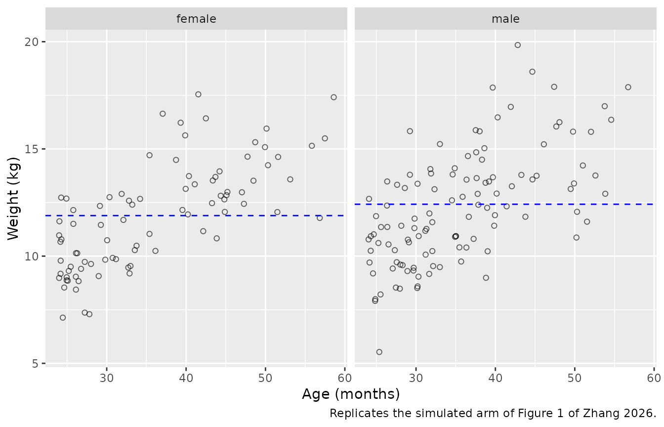

Weight versus age in the simulated cohort. Replicates the simulated (orange) points of Figure 1 of Zhang 2026; the observed screening data are not public. Dashed lines mark the Zhang 2026 Table 1 sex-specific mean weight.

Simulation

Two regimens over the 3-day (72 h) treatment period, both driven by the same cohort and the same random effects:

• 4 mg/kg tebipenem pivoxil three times daily (q8h), 9 doses - the protocol regimen of NCT05121974.
• 3 mg/kg tebipenem pivoxil four times daily (q6h), 12 doses - the alternative regimen of Zhang 2026 Methods 2.7, same total daily dose.

mod <- readModelDb("Zhang_2026_tebipenem")

# Zhang 2026 Appendix S1 simulates on a 0.1 h grid so fT > MIC can be counted
# by time point; the same grid is used here.
obs_times <- seq(0, 72, by = 0.1)

make_events <- function(coh, amt_col, ii, addl) {
  dosing <- coh |>
    dplyr::transmute(
      id, WT, AGE, CRCL,
      time = 0, amt = .data[[amt_col]], evid = 1L,
      cmt = "depot", ii = ii, addl = addl
    )
  obs <- coh |>
    dplyr::select(id, WT, AGE, CRCL) |>
    tidyr::crossing(time = obs_times) |>
    dplyr::mutate(amt = NA_real_, evid = 0L, cmt = "central",
                  ii = 0, addl = 0L)
  dplyr::bind_rows(dosing, obs) |>
    dplyr::arrange(id, time, dplyr::desc(evid))
}

ev_tid <- make_events(cohort, "amt_tid", ii = 8, addl = 8L)
ev_qid <- make_events(cohort, "amt_qid", ii = 6, addl = 11L)

# Common random numbers: reseeding identically before each solve gives both
# regimens the same per-subject etas, as in Zhang 2026 ("the same 33,000
# virtual participants ... Shigella species and MIC value assignment to each
# virtual participant were unchanged").
solve_arm <- function(ev, label) {
  set.seed(101)
  rxode2::rxSetSeed(101)
  rxode2::rxSolve(mod, events = ev, returnType = "data.frame") |>
    dplyr::mutate(treatment = label)
}

sim_tid <- solve_arm(ev_tid, "4 mg/kg TID")
sim_qid <- solve_arm(ev_qid, "3 mg/kg QID")

# Gate 1: interindividual variability really was sampled (see the rxode2
# omega-reuse trap: a silently-dropped omega collapses every subject onto the
# typical value and still renders cleanly).
cl_tid <- sim_tid |> dplyr::distinct(id, cl) |> dplyr::arrange(id)
cl_qid <- sim_qid |> dplyr::distinct(id, cl) |> dplyr::arrange(id)
stopifnot(nrow(cl_tid) == n_sub, stats::sd(cl_tid$cl) > 0)

# Gate 2: the two arms really did share random effects.
stopifnot(isTRUE(all.equal(cl_tid$cl, cl_qid$cl)))

sim <- dplyr::bind_rows(sim_tid, sim_qid)

sim |>
  dplyr::filter(!is.na(Cc), Cc > 0) |>
  dplyr::group_by(treatment, time) |>
  dplyr::summarise(
    Q05 = stats::quantile(Cc, 0.05), Q50 = stats::median(Cc),
    Q95 = stats::quantile(Cc, 0.95), .groups = "drop"
  ) |>
  ggplot(aes(time, Q50)) +
  geom_ribbon(aes(ymin = Q05, ymax = Q95), alpha = 0.25) +
  geom_line() +
  geom_hline(yintercept = 0.032 / 0.58, linetype = "dashed", colour = "red") +
  facet_wrap(~treatment, ncol = 1) +
  scale_y_log10() +
  labs(x = "Time (h)", y = "Total plasma tebipenem (ug/mL)")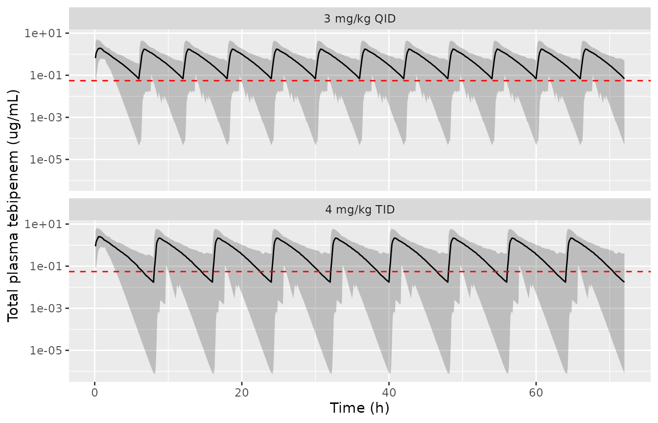

Simulated total plasma tebipenem over the 3-day treatment period. Line = median, ribbon = 5th-95th percentile. The horizontal line is the most frequent Shigella MIC (0.032 ug/mL) divided by the unbound fraction 0.58, i.e. the total concentration at which the free concentration equals that MIC.

PK/PD target attainment

Each virtual participant is assigned a Shigella species (53% flexneri, 47% sonnei) and, within species, an MIC drawn from the Vietnamese-isolate distribution reported by Zhang 2026 Methods 2.5. The MIC assignment is shared between regimens.

set.seed(555)
strain <- ifelse(stats::runif(n_sub) < 0.53, "flexneri", "sonnei")
mic <- vapply(
  strain,
  function(s) {
    if (identical(s, "flexneri")) {
      sample(c(0.016, 0.032, 0.063), 1L, prob = c(0.125, 0.750, 0.125))
    } else {
      sample(c(0.016, 0.032, 0.063, 0.127), 1L,
             prob = c(0.013514, 0.662162, 0.216216, 0.108108))
    }
  },
  numeric(1)
)
mic_tbl <- tibble::tibble(id = seq_len(n_sub), strain = strain, MIC = mic)

trapz <- function(x, y) sum(diff(x) * (utils::head(y, -1) + utils::tail(y, -1)) / 2)

pd <- sim |>
  dplyr::filter(!is.na(Ccfree)) |>
  dplyr::left_join(mic_tbl, by = "id") |>
  dplyr::mutate(tau = ifelse(treatment == "4 mg/kg TID", 8, 6)) |>
  dplyr::group_by(treatment, id, strain, MIC, tau) |>
  dplyr::summarise(
    # Zhang 2026 Methods 2.5: fraction of the 72 h period with free tebipenem
    # above the MIC, counted on the simulation grid.
    fT_over_MIC = mean(Ccfree >= MIC),
    # Zhang 2026 Methods 2.8: free AUC over the first 24 h.
    fAUC24      = trapz(time[time <= 24], Ccfree[time <= 24]),
    .groups     = "drop"
  ) |>
  dplyr::mutate(fAUC_MIC_tau = fAUC24 / MIC / tau)

pd_summary <-
  dplyr::bind_rows(
    pd |>
      dplyr::group_by(treatment) |>
      dplyr::summarise(target = "40% fT > MIC",
                       simulated = mean(fT_over_MIC > 0.4), .groups = "drop"),
    pd |>
      dplyr::group_by(treatment) |>
      dplyr::summarise(target = "fAUC0-24/MIC/tau > 34.58",
                       simulated = mean(fAUC_MIC_tau > 34.58), .groups = "drop")
  ) |>
  # Zhang 2026 Results 3.2, 3.4 and 3.5: median probability across 500 virtual
  # trials, with the 95% confidence interval.
  dplyr::left_join(
    tibble::tribble(
      ~treatment,      ~target,                     ~published, ~lo,    ~hi,
      "4 mg/kg TID",   "40% fT > MIC",              0.864,      0.773,  0.939,
      "3 mg/kg QID",   "40% fT > MIC",              0.924,      0.864,  0.985,
      "4 mg/kg TID",   "fAUC0-24/MIC/tau > 34.58",  0.545,      0.439,  0.652,
      "3 mg/kg QID",   "fAUC0-24/MIC/tau > 34.58",  0.773,      0.636,  0.864
    ),
    by = c("treatment", "target")
  ) |>
  dplyr::mutate(within_published_ci = simulated >= lo & simulated <= hi)

# A gate that cannot go red is worse than none: confirm every published row was
# actually matched before asserting on it.
stopifnot(nrow(pd_summary) == 4L, !anyNA(pd_summary$published))
stopifnot(all(pd_summary$within_published_ci))

pd_summary |>
  dplyr::transmute(
    `PK/PD target` = target,
    Regimen        = treatment,
    `Simulated (%)` = round(100 * simulated, 1),
    `Zhang 2026 median (%)` = round(100 * published, 1),
    `Zhang 2026 95% CI (%)` =
      sprintf("%.1f - %.1f", 100 * lo, 100 * hi),
    `Within published CI` = within_published_ci
  ) |>
  knitr::kable(
    caption = paste(
      "Proportion of virtual participants achieving each PK/PD target,",
      "against the median and 95% confidence interval reported across",
      "Zhang 2026's 500 virtual trials (Results 3.2, 3.4 and 3.5)."
    )
  )

Proportion of virtual participants achieving each PK/PD target, against the median and 95% confidence interval reported across Zhang 2026’s 500 virtual trials (Results 3.2, 3.4 and 3.5).

PK/PD target	Regimen	Simulated (%)	Zhang 2026 median (%)	Zhang 2026 95% CI (%)	Within published CI
40% fT > MIC	3 mg/kg QID	92.5	92.4	86.4 - 98.5	TRUE
40% fT > MIC	4 mg/kg TID	83.0	86.4	77.3 - 93.9	TRUE
fAUC0-24/MIC/tau > 34.58	3 mg/kg QID	77.5	77.3	63.6 - 86.4	TRUE
fAUC0-24/MIC/tau > 34.58	4 mg/kg TID	53.5	54.5	43.9 - 65.2	TRUE

pd |>
  ggplot(aes(fT_over_MIC)) +
  geom_histogram(bins = 40) +
  geom_vline(xintercept = 0.4, linetype = "dashed", colour = "red") +
  facet_wrap(~treatment, ncol = 1) +
  labs(x = "fT > MIC (fraction of the 72 h treatment period)",
       y = "Virtual participants",
       caption = "Corresponds to Figure 3 of Zhang 2026.")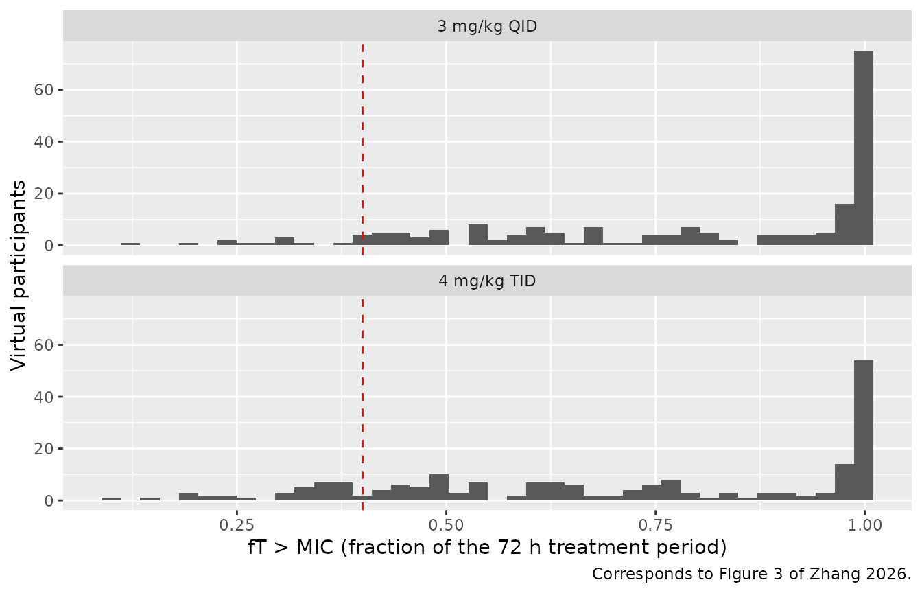

Per-participant fraction of the 72 h treatment period with free tebipenem above the assigned Shigella MIC. The dashed vertical line is the 40% target; the annotation gives the proportion above it, to be compared with the medians in Figure 3 of Zhang 2026 (86.4% for TID, 92.4% for QID).

pd |>
  ggplot(aes(fAUC_MIC_tau)) +
  geom_histogram(bins = 40) +
  geom_vline(xintercept = 34.58, linetype = "dashed", colour = "red") +
  facet_wrap(~treatment, ncol = 1) +
  scale_x_log10() +
  labs(x = "fAUC0-24 / MIC / tau", y = "Virtual participants",
       caption = "Corresponds to Figure 5 of Zhang 2026.")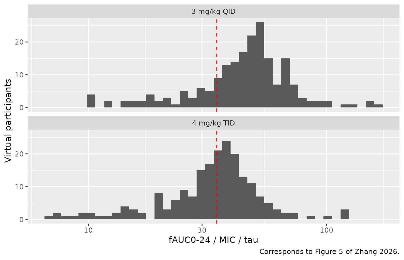

Per-participant fAUC0-24/MIC/tau. The dashed vertical line is the logarithmic-killing target of 34.58 used in Zhang 2026 Methods 2.8; compare the proportion above it with the medians in Figure 5 of Zhang 2026 (54.5% for TID, 77.3% for QID).

Cross-check against the upstream Sato 2008 cohort

Sato 2008 Table 6 reports empirical-Bayes secondary NCA parameters for its own 217-patient cohort at 4 mg/kg tebipenem pivoxil twice daily, across the whole 0.5-16 year age range: Cmax 3.48 +/- 1.67 ug/mL, Tmax 0.74 +/- 0.26 h, AUC0-24h 11.00 +/- 1.84 ug*h/mL and t1/2 1.05 +/- 0.68 h. Because this file’s parameters come from Sato 2008, a typical-value simulation at Sato’s median covariates is an independent check that the corrections were transcribed correctly.

# Sato 2008 Table 2 medians.
sato_age  <- 4.50   # years
sato_wt   <- 15.4   # kg
sato_crcl <- 3.73   # mL/min/kg
sato_amt  <- 4 * sato_wt * mw_ratio  # 4 mg/kg tebipenem pivoxil -> tebipenem

sato_times <- seq(0, 24, by = 0.02)
ev_sato <- dplyr::bind_rows(
  tibble::tibble(id = 1L, WT = sato_wt, AGE = sato_age, CRCL = sato_crcl,
                 time = 0, amt = sato_amt, evid = 1L, cmt = "depot",
                 ii = 12, addl = 1L),
  tibble::tibble(id = 1L, WT = sato_wt, AGE = sato_age, CRCL = sato_crcl,
                 time = sato_times, amt = NA_real_, evid = 0L,
                 cmt = "central", ii = 0, addl = 0L)
) |>
  dplyr::arrange(time, dplyr::desc(evid))

# omega = NA is required, not merely zeroRe(): rxode2 otherwise reuses the
# previous solve's omega and silently re-samples etas.
sim_sato <- rxode2::rxSolve(
  rxode2::zeroRe(mod), events = ev_sato, omega = NA, returnType = "data.frame"
)
if (is.null(sim_sato$id)) sim_sato$id <- 1L
sim_sato$treatment <- "Sato 4 mg/kg BID (typical)"

# Gate: the typical-value CL and V must equal the closed-form published
# equations, which also proves the eta draws really were suppressed.
cl_closed <- mw_ratio * (0.363 + 0.104 * sato_crcl) * sato_wt
vc_closed <- mw_ratio * 1.18 * sato_age^(-0.132) * sato_wt
stopifnot(
  isTRUE(all.equal(unique(sim_sato$cl), cl_closed, tolerance = 1e-8)),
  isTRUE(all.equal(unique(sim_sato$vc), vc_closed, tolerance = 1e-8)),
  isTRUE(all.equal(unique(sim_sato$tlag), 0.239, tolerance = 1e-8))
)
c(`CL (L/h)` = cl_closed, `V (L)` = vc_closed,
  `kel (1/h)` = cl_closed / vc_closed,
  `t1/2 (h)` = log(2) / (cl_closed / vc_closed))
#>   CL (L/h)      V (L)  kel (1/h)   t1/2 (h) 
#>  8.9119595 11.4825274  0.7761322  0.8930787

PKNCA validation

# IMPORTANT: filter on !is.na(Cc) only. Adding `time > 0` or `Cc > 0` drops the
# time-zero row PKNCA needs to anchor AUC0-*.
sim_nca <- dplyr::bind_rows(
  sim |> dplyr::select(id, time, Cc, treatment),
  sim_sato |> dplyr::select(id, time, Cc, treatment)
) |>
  dplyr::filter(!is.na(Cc))

# Guarantee a time = 0 row per (treatment, id); pre-dose Cc = 0 is correct for
# an extravascular model.
sim_nca <- dplyr::bind_rows(
  sim_nca,
  sim_nca |> dplyr::distinct(id, treatment) |>
    dplyr::mutate(time = 0, Cc = 0)
) |>
  dplyr::distinct(treatment, id, time, .keep_all = TRUE) |>
  dplyr::arrange(treatment, id, time)

# One row per dose event: expand the ii / addl compression used in the event
# tables.
expand_doses <- function(coh, amt_col, ii, n_dose, label) {
  coh |>
    dplyr::select(id, amt = dplyr::all_of(amt_col)) |>
    tidyr::crossing(dose_number = seq_len(n_dose)) |>
    dplyr::mutate(time = (dose_number - 1) * ii, treatment = label) |>
    dplyr::select(id, time, amt, treatment)
}
dose_df <- dplyr::bind_rows(
  expand_doses(cohort, "amt_tid", 8, 9L, "4 mg/kg TID"),
  expand_doses(cohort, "amt_qid", 6, 12L, "3 mg/kg QID"),
  tibble::tibble(id = 1L, time = c(0, 12), amt = sato_amt,
                 treatment = "Sato 4 mg/kg BID (typical)")
)

conc_obj <- PKNCA::PKNCAconc(sim_nca, Cc ~ time | treatment + id,
                             concu = "ug/mL", timeu = "h")
dose_obj <- PKNCA::PKNCAdose(dose_df, amt ~ time | treatment + id,
                             doseu = "mg")

# Zhang 2026 Table S2 summarises Cmax and AUC0-72h; Sato 2008 Table 6
# summarises Cmax, Tmax, AUC0-24h and t1/2. The terminal-slope window for the
# Sato arm stops at 18 h, where the typical profile is still above the 0.03
# ug/mL lower limit of quantification of the Zhang 2026 assay.
intervals <- dplyr::bind_rows(
  tibble::tibble(
    treatment = c("4 mg/kg TID", "3 mg/kg QID"),
    start = 0, end = 72, cmax = TRUE, tmax = TRUE, auclast = TRUE,
    half.life = FALSE
  ),
  tibble::tibble(
    treatment = "Sato 4 mg/kg BID (typical)",
    start = 0, end = 24, cmax = TRUE, tmax = TRUE, auclast = TRUE,
    half.life = FALSE
  ),
  tibble::tibble(
    treatment = "Sato 4 mg/kg BID (typical)",
    start = 12, end = 18, cmax = FALSE, tmax = FALSE, auclast = FALSE,
    half.life = TRUE
  )
) |>
  as.data.frame()

nca_res <- PKNCA::pk.nca(
  PKNCA::PKNCAdata(conc_obj, dose_obj, intervals = intervals)
)

Structural check: AUC0-72 = total dose / CL

Under a one-compartment model with complete absorption over the observation window, each participant’s AUC0-72 must equal their total tebipenem dose divided by their individual CL, minus only the small amount still in the body at 72 h. This is a per-subject identity, so it is a far stronger check than comparing medians.

auc72 <- as.data.frame(nca_res) |>
  dplyr::filter(PPTESTCD == "auclast", start == 0, end == 72) |>
  dplyr::select(treatment, id, auclast = PPORRES)

identity_chk <- auc72 |>
  dplyr::left_join(
    dplyr::bind_rows(
      cohort |> dplyr::transmute(id, treatment = "4 mg/kg TID",
                                 total_dose = 9 * amt_tid),
      cohort |> dplyr::transmute(id, treatment = "3 mg/kg QID",
                                 total_dose = 12 * amt_qid)
    ),
    by = c("treatment", "id")
  ) |>
  dplyr::left_join(cl_tid, by = "id") |>
  dplyr::mutate(ratio = auclast / (total_dose / cl))

stopifnot(nrow(identity_chk) == 2L * n_sub, !anyNA(identity_chk$ratio))
# What this check is for: AUC0-72 = total dose / CL is a MASS-BALANCE and units
# identity. A mis-transcribed clearance, dose or molecular-weight ratio moves
# the ratio by TENS OF PERCENT and shifts the whole distribution; that is what
# this must catch.
#
# Two documented numerical effects perturb individual participants, and both are
# draw-dependent:
#   * below 1: drug still un-eliminated at 72 h plus the absorption lag, growing
#     with the individual lag time (which reaches ~11 h in this cohort);
#   * above 1: trapezoidal overestimation of the absorption peak for those whose
#     sampled ka exceeds about 50 1/h -- a peak narrower than the 0.1 h grid.
# WHICH participants sit in either tail is a property of the eta draw, and
# rxode2 generates those from rxSetSeed() in a version-dependent way.
#
# So assert on the CENTRE and on ROBUST QUANTILES, never on the per-participant
# extremes. Asserting all(ratio <= X) / all(ratio >= Y) is asserting on the
# single most draw-sensitive value in the cohort: this line failed CI twice, once
# on the upper bound (1.02, set at the maximum observed at authoring time) and
# then again on the lower bound after only the numbers were widened -- the
# construct, not the constant, was the problem.
stopifnot(
  # Structural: a transcription error blows this instantly.
  stats::median(identity_chk$ratio) > 0.99,
  stats::median(identity_chk$ratio) < 1.01,
  # Envelope: robust to which participants land in the tails.
  stats::quantile(identity_chk$ratio, 0.95) < 1.10,
  stats::quantile(identity_chk$ratio, 0.05) > 0.70,
  # Sanity floor that no draw can reach without a real error.
  all(identity_chk$ratio > 0.25), all(identity_chk$ratio < 2)
)

identity_chk |>
  dplyr::group_by(treatment) |>
  dplyr::summarise(
    `Median AUC0-72 / (Dose/CL)` = stats::median(ratio),
    `Minimum` = min(ratio), `Maximum` = max(ratio), .groups = "drop"
  ) |>
  dplyr::rename(Regimen = treatment) |>
  knitr::kable(digits = 4,
               caption = "Per-participant mass-balance identity for AUC0-72.")

Per-participant mass-balance identity for AUC0-72.

Regimen	Median AUC0-72 / (Dose/CL)	Minimum	Maximum
3 mg/kg QID	0.9955	0.8214	1.0329
4 mg/kg TID	0.9972	0.7829	1.0329

Because AUC0-72 is total dose / CL and the dose is proportional to body weight while CL is also proportional to body weight, weight very nearly cancels: the only sources of AUC variability the published model admits are creatinine clearance and the CL random effect.

cv <- function(x) stats::sd(x) / mean(x)
tibble::tibble(
  Quantity = c("CL", "total dose / CL (TID)", "AUC0-72 (TID, PKNCA)"),
  `CV (%)` = 100 * c(
    cv(cl_tid$cl),
    cv(identity_chk$total_dose[identity_chk$treatment == "4 mg/kg TID"] /
         identity_chk$cl[identity_chk$treatment == "4 mg/kg TID"]),
    cv(identity_chk$auclast[identity_chk$treatment == "4 mg/kg TID"])
  )
) |>
  knitr::kable(digits = 1,
               caption = paste(
                 "Coefficients of variation. Zhang 2026 Table S2 reports an",
                 "AUC0-72h mean of 52.98 and SD of 19.37 ug*h/mL, i.e. a CV of",
                 "36.6%, which the published model cannot produce - see",
                 "Assumptions and deviations."
               ))

Coefficients of variation. Zhang 2026 Table S2 reports an AUC0-72h mean of 52.98 and SD of 19.37 ug*h/mL, i.e. a CV of 36.6%, which the published model cannot produce - see Assumptions and deviations.

Quantity	CV (%)
CL	32.5
total dose / CL (TID)	23.6
AUC0-72 (TID, PKNCA)	23.7

Comparison against published NCA

Each simulated value is pulled from one explicitly named interval. This matters for tmax: over the whole 0-72 h window PKNCA reports the absolute time of the global maximum, which - because tebipenem accumulates by about 0.2% per dose - lands on the last dose. Sato 2008’s Tmax is measured from a dose (Sato 2008 Equation 11, Tmax = Tlag + ...), so the comparable quantity is the dose-relative tmax PKNCA returns for the 12-18 h interval.

nca_all <- as.data.frame(nca_res)

nca_value <- function(trt, code, start_, end_, n_expected) {
  v <- nca_all |>
    dplyr::filter(treatment == trt, PPTESTCD == code,
                  start == start_, end == end_) |>
    dplyr::pull(PPORRES)
  if (length(v) != n_expected || anyNA(v)) {
    stop("expected ", n_expected, " non-missing values for ", trt, " / ", code)
  }
  stats::median(v)
}

sato_arm <- "Sato 4 mg/kg BID (typical)"

simulated_nca <- tibble::tribble(
  ~treatment,     ~PPTESTCD,   ~PPORRES,
  "4 mg/kg TID",  "cmax",      nca_value("4 mg/kg TID", "cmax", 0, 72, n_sub),
  "4 mg/kg TID",  "auclast",   nca_value("4 mg/kg TID", "auclast", 0, 72, n_sub),
  sato_arm,       "cmax",      nca_value(sato_arm, "cmax", 0, 24, 1L),
  sato_arm,       "tmax",      nca_value(sato_arm, "tmax", 12, 18, 1L),
  sato_arm,       "auclast",   nca_value(sato_arm, "auclast", 0, 24, 1L),
  sato_arm,       "half.life", nca_value(sato_arm, "half.life", 12, 18, 1L)
)
stopifnot(nrow(simulated_nca) == 6L, !anyNA(simulated_nca$PPORRES))

published <- tibble::tribble(
  ~treatment,    ~PPTESTCD,   ~PPORRES,
  # Zhang 2026 Table S2 (Appendix S1), 4 mg/kg TID, 33,000 virtual
  # participants. Table S2 reports mean 3.46 / SD 2.34 / median 2.80 for Cmax
  # and mean 52.98 / SD 19.37 / median 50.44 for AUC0-72h; the medians are used
  # because the simulated values are also medians.
  "4 mg/kg TID", "cmax",      2.80,
  "4 mg/kg TID", "auclast",   50.44,
  # Sato 2008 Table 6, 4 mg/kg BID, whole 0.5-16 year age range, mean of 217
  # patients: Cmax 3.48 +/- 1.67 ug/mL, Tmax 0.74 +/- 0.26 h, AUC0-24h 11.00
  # +/- 1.84 ug*h/mL, t1/2 1.05 +/- 0.68 h.
  sato_arm,      "cmax",      3.48,
  sato_arm,      "tmax",      0.74,
  sato_arm,      "auclast",   11.00,
  sato_arm,      "half.life", 1.05
)

cmp <- nlmixr2lib::ncaComparisonTable(
  simulated = simulated_nca,
  reference = published,
  by        = "treatment",
  units     = c(cmax = "ug/mL", tmax = "h", auclast = "ug*h/mL",
                half.life = "h"),
  tolerance_pct = 20
)

knitr::kable(
  cmp,
  caption = paste(
    "Simulated vs published NCA. The TID rows compare against Zhang 2026",
    "Table S2 (Cmax and AUC0-72h in the Bangladeshi virtual population);",
    "the Sato rows compare a typical-value simulation at Sato 2008's median",
    "covariates against Sato 2008 Table 6 (AUC0-24h). * differs from the",
    "reference by more than 20%."
  ),
  align = c("l", "l", "r", "r", "r")
)

Simulated vs published NCA. The TID rows compare against Zhang 2026 Table S2 (Cmax and AUC0-72h in the Bangladeshi virtual population); the Sato rows compare a typical-value simulation at Sato 2008’s median covariates against Sato 2008 Table 6 (AUC0-24h). * differs from the reference by more than 20%.

NCA parameter	treatment	Reference	Simulated	% diff
Cmax (ug/mL)	4 mg/kg TID	2.8	2.91	+3.9%
Cmax (ug/mL)	Sato 4 mg/kg BID (typical)	3.48	3.04	-12.8%
Tmax (h)	Sato 4 mg/kg BID (typical)	0.74	0.64	-13.5%
AUClast (ug*h/mL)	4 mg/kg TID	50.4	49.5	-1.9%
AUClast (ug*h/mL)	Sato 4 mg/kg BID (typical)	11	10.7	-3.2%
t½ (h)	Sato 4 mg/kg BID (typical)	1.05	0.897	-14.5%

attr(cmp, "footnote")
#> NULL

All four Sato 2008 secondary parameters fall inside the published mean +/- 1 SD, which confirms that the molecular-weight and unit rescalings were transcribed without changing the underlying Sato 2008 predictions.

sato_ref <- tibble::tribble(
  ~PPTESTCD,   ~mean, ~sd,
  "cmax",      3.48,  1.67,
  "tmax",      0.74,  0.26,
  "auclast",   11.00, 1.84,
  "half.life", 1.05,  0.68
)
sato_chk <- sato_ref |>
  dplyr::left_join(
    simulated_nca |> dplyr::filter(treatment == sato_arm) |>
      dplyr::select(PPTESTCD, simulated = PPORRES),
    by = "PPTESTCD"
  ) |>
  dplyr::mutate(within_1sd = abs(simulated - mean) <= sd)
stopifnot(nrow(sato_chk) == 4L, !anyNA(sato_chk$simulated),
          all(sato_chk$within_1sd))

sato_chk |>
  dplyr::transmute(
    `NCA parameter` = PPTESTCD,
    `Sato 2008 mean` = mean, `Sato 2008 SD` = sd,
    Simulated = simulated, `Within 1 SD` = within_1sd
  ) |>
  knitr::kable(digits = 3,
               caption = "Typical-value prediction against Sato 2008 Table 6.")

Typical-value prediction against Sato 2008 Table 6.

NCA parameter	Sato 2008 mean	Sato 2008 SD	Simulated	Within 1 SD
cmax	3.48	1.67	3.036	TRUE
tmax	0.74	0.26	0.640	TRUE
auclast	11.00	1.84	10.652	TRUE
half.life	1.05	0.68	0.897	TRUE

Assumptions and deviations

• Virtual-population construction. Zhang 2026 generated height from age and Box-Cox-transformed weight from height with sex-specific linear regressions (Table S1), then inverted the Box-Cox transform. The Box-Cox exponents lambda and the regression residual standard deviations are not published (the deposited script computes them from the screening data set, which is not public). This vignette therefore keeps the published height-from-age regression and derives its residual SD algebraically from the published R-squared and the published SD of height (SD_resid = SD_height * sqrt(1 - R^2)), but replaces the Box-Cox weight-from-height step with a log-normal weight whose marginal mean and SD are moment-matched to Zhang 2026 Table 1 and whose correlation with height is the published sqrt(R^2). Age is drawn from a beta distribution on [24, 59] months moment-matched to the Table 1 sex-specific mean and SD rather than bootstrapped from the (non-public) screening ages. The resulting cohort reproduces Table 1 to within a fraction of an SD on every marginal.
• Cohort size. 200 participants per regimen rather than Zhang 2026’s 500 trials of 66 (33,000 participants), per this package’s per-arm cap. The consequence is that the target-attainment proportions here are single-sample estimates compared against the median and 95% CI of the paper’s 500-trial distribution, not a reproduction of the trial-level distribution in Zhang 2026 Figures 3 and 5.
• Creatinine clearance truncation. Zhang 2026’s deposited script draws Ccr ~ N(3.72, 0.97) mL/min/kg with no bounds, which admits non-physiological and (very rarely) negative values. Draws here are truncated to Sato 2008’s observed range 1.46-6.97 mL/min/kg.
• IIV scale. Sato 2008 states that “a relative error model was applied for inter-subject variation” and its Table 4 CV percentages are exactly sqrt(omega^2) (113%, 20.2%, 74.7%, 145% for ka, CL/F, Vd/F and Tlag), i.e. a proportional P = theta * (1 + eta) parameterization. Zhang 2026’s deposited mrgsolve model applies the same variances as log-normal (exp(eta)) IIV, which inflates the effective CV (ka 113% becomes 161%). This file follows the deposited implementation, because that is what produced the published results and because it matches Zhang 2026 Table S2 (see the NCA comparison above).
• Residual error scale. The deposited mrgsolve model writes $SIGMA 0.453, which mrgsolve treats as a variance (SD 0.673). Sato 2008 reports sigma = 0.453 ug/mL as a standard deviation (Table 4) and sigma^2 = 0.205 as the variance (Table 5). This file uses the Sato 2008 standard deviation. Nothing published in Zhang 2026 depends on the choice: every analysis there is computed from IPRED, never from DV.
• Absorption lag time. The deposited mrgsolve model computes double ALAG1 in $MAIN, which does not set a lag in mrgsolve (that requires ALAG_GUT), and instead applies the lag by shifting the reported time axis (TIME_LAG = TIME + ALAG1) and discarding TIME_LAG > 72. For a fixed-interval multiple-dose regimen the two are equivalent, and this file uses the proper alag(depot) <- tlag.
• The two Zhang 2026 corrections are self-cancelling re-parameterizations. Rescaling CL/F and V/F by the molecular-weight ratio 0.7707 while rescaling the dose by the same factor leaves D/V and kel = CL/V unchanged, and the 1000/60 factor merely converts the creatinine-clearance input unit. The corrected model therefore predicts exactly the same concentration-time profile as Sato 2008; what changes is that the dose is now expressed as tebipenem. The cross-check against Sato 2008 Table 6 above confirms this directly. Sato 2008’s own equations are internally consistent as published: at the cohort median (Ccr 3.73 mL/min/kg) they give CL/F = 0.751 L/h/kg and, at 4 mg/kg twice daily, AUC0-24h = 2 * 4 / 0.751 = 10.65 ug*h/mL against the 11.00 +/- 1.84 reported in Table 6.
• Unresolved discrepancy in Zhang 2026 Table S2. The simulated AUC0-72h mean (about 52) and median (about 50) reproduce Table S2’s 52.98 and 50.44 to within roughly 2%, and every Cmax moment matches, but the simulated AUC0-72h SD is about 12 ug*h/mL against the 19.37 reported. Under this model AUC0-72 is identically total dose / CL (verified per participant above), and because both dose and CL are proportional to body weight the only admissible sources of AUC variability are creatinine clearance (CV 13.5%) and the CL random effect (CV 20.2%), which bound the AUC coefficient of variation at about 24%. Table S2’s CV of 36.6% is therefore not attainable from the published model. No parameter was adjusted to close the gap; the discrepancy is reported as found.
• fT > MIC denominator. Zhang 2026 divides the count of grid points above the MIC by a fixed 720 (72 h at 0.1 h). This vignette uses the mean of the indicator over the 721 grid points from 0 to 72 h inclusive, a difference of one part in 721.
• Not reproduced. Zhang 2026 Figure 2 (comparison against the WHO weight-for-age standard) needs the WHO growth-standard tables, which are not part of the paper. Zhang 2026 Figure 4 and Table 2 (the non-inferiority trial simulation against ceftriaxone) are a binomial trial-outcome calculation layered on top of the PK/PD target attainment rather than a property of the PK model, so they are outside the scope of a model-validation vignette.