Vancomycin (Alqurain 2024)
Source:vignettes/articles/Alqurain_2024_vancomycin.Rmd
Alqurain_2024_vancomycin.Rmd
ui <- rxode2::rxode(readModelDb("Alqurain_2024_vancomycin"))
#> ℹ parameter labels from comments will be replaced by 'label()'
Model and source
- Citation: Alqurain AA, Alrashidi LN, Aloraifej SK, Alkhalifah M, Alsayed HA, Abohelaika S, Alshabeeb MA, Aldhafeeri AS, Almuslim M, Bumozah TN, Alomar MJ, Alshehab AA, Alamer AA, Al-Matouq J, Bidasee KR, Alomar FA. Factors Affecting Vancomycin Trough Concentration; a Population Pharmacokinetic Model in Non-Critical Care Saudi Patients. Drug Des Devel Ther. 2024;18:6185-6198. doi:10.2147/DDDT.S496512
- Description: One-compartment IV population PK model for vancomycin in non-critical-care adult (>= 40 years) medical-ward inpatients in the Eastern Province of Saudi Arabia, built from routine therapeutic-drug-monitoring trough concentrations. Clearance is an uncentered exponential (log-linear) function of C-reactive protein and Cockcroft-Gault creatinine clearance, so exp(lcl) is the clearance at CRP = 0 and CRCL = 0 rather than a typical-patient clearance; volume of distribution carries no covariates.
- Article: https://doi.org/10.2147/DDDT.S496512
- Supplement (Supplementary Tables 1-9, Supplementary Figure 1): https://www.dovepress.com/get_supplementary_file.php?f=496512.docx
Alqurain 2024 is a multicentre retrospective population-PK analysis of routine vancomycin therapeutic-drug-monitoring records from three hospitals in the Eastern Province of Saudi Arabia. Because the dataset consists exclusively of trough concentrations drawn as part of routine TDM, the authors could not resolve a distribution phase; a one-compartment model with linear elimination and IV input was retained on AIC grounds over two- and three-compartment, lag-time, and Michaelis-Menten alternatives (Supplementary Tables 1-6).
Population
pop <- ui$population
tibble::tibble(Field = names(pop), Value = vapply(pop, paste, character(1), collapse = "; ")) |>
knitr::kable(caption = "Study population (Alqurain 2024 Table 1).")| Field | Value |
|---|---|
| species | human |
| n_subjects | 124 |
| n_observations | 172 |
| n_studies | 1 |
| age_range | 40-99 years (inclusion criterion >= 40 years); median 79 years (IQR 50-86). Age bands (Table 1): 40-49 8 (7%), 50-59 8 (7%), 60-69 42 (33%), 70-79 31 (25%), 80-89 26 (21%), 90-99 9 (7%). |
| age_median | 79 years |
| weight_range | Mean 72 +/- 20 kg (Table 1) |
| sex_female_pct | 41 |
| race_ethnicity | Not reported; single-country cohort recruited in the Eastern Province of Saudi Arabia |
| disease_state | Adults admitted to general medical wards and initiated on systemic vancomycin. Patients in the emergency department, intensive care unit or surgical wards, patients with chronic kidney disease, and pregnant women were excluded, so this is explicitly a non-critical-care population. Most patients nonetheless had some degree of (acute) renal impairment: mean CrCl 61.1 +/- 48.2 mL/min, 35% at <= 30 mL/min. Mean serum albumin 29.5 +/- 8 g/L; mean serum creatinine 183 +/- 171 (units reported as mg/dL in Table 1, but the magnitude is consistent with umol/L). |
| renal_function | Mean Cockcroft-Gault CrCl 61.1 +/- 48.2 mL/min; > 120 mL/min 17 (14%), 91-120 21 (17%), 61-90 14 (11%), 31-60 28 (23%), <= 30 mL/min 44 (35%) (Table 1) |
| dose_range | 500-1750 mg per intravenous dose (Table 1: 500 mg 25%, 750 mg 15%, 850 mg 2%, 1000 mg 40%, 1200 mg 1%, 1250 mg 9%, 1500 mg 6%, 1750 mg 2%). Doses were standardized to 500 mg for figure presentation only; actual doses were used in the modelling. |
| regions | Saudi Arabia (Eastern Province): Al-Mana General Hospital Al-Khobar, Qatif Central Hospital, and Dammam Medical Complex |
| notes | Multicentre retrospective study of routine therapeutic-drug-monitoring records collected 1 January - 31 December 2022; one visit per patient. 172 trough concentrations from 124 patients. Baseline demographics are Table 1 of Alqurain 2024. Concentrations were measured by enzyme-multiplied immunoassay (EMIT) with a 2-50 mg/L calibration range, so only trough samples inform the fit – the authors note this prevented resolution of a distribution phase and is why a one-compartment model was retained. |
172 vancomycin trough concentrations from 124 patients aged 40 years and older (median 79) admitted to general medical wards between 1 January and 31 December 2022. Patients in the emergency department, intensive care unit or surgical wards, those with chronic kidney disease, and pregnant women were excluded, so this is explicitly a non-critical-care cohort. Renal function was nonetheless substantially impaired in most patients: mean Cockcroft-Gault CrCl 61.1 +/- 48.2 mL/min, with 35% at or below 30 mL/min. Mean body weight was 72 +/- 20 kg and 41% of the cohort were women. Intravenous doses ranged from 500 to 1750 mg, with 1000 mg the most common (40%). Concentrations were assayed by enzyme-multiplied immunoassay (EMIT) over a 2-50 mg/L calibration range.
The same information is available programmatically via
readModelDb("Alqurain_2024_vancomycin")()$population.
Source trace
Every ini() entry in
inst/modeldb/specificDrugs/Alqurain_2024_vancomycin.R
carries an in-file comment naming its source location. They are
collected here for review.
| Equation / parameter | Value | Source location |
|---|---|---|
lvc (V) |
193.65 L (RSE 7.41%) | Table 2, “Final Model / Population” column, row
V (L)
|
lcl (CL intercept) |
3.52 L/h (RSE 62.5%) | Table 2, “Final Model / Population” column, row
CL (L/h)
|
e_crp_cl |
-0.05 per mg/L (RSE 28%) | Table 2, “Final Model / Population” column, row
CRP effect on CL
|
e_crcl_cl |
0.0088 per mL/min (RSE 48.4%) | Table 2, “Final Model / Population” column, row
CrCl effect on CL
|
etalvc |
variance 0.1089 (= 0.33^2) | Table 2, row Omega V = 0.33; Table 2 footnote: “Omega,
Inter-individual variability presented as standard deviation” |
etalcl |
variance 0.6561 (= 0.81^2) | Table 2, row Omega Cl = 0.81; same footnote.
Cross-checks against the Results text “reduction in BSV for CL from 173%
to 81%” (= 100 x omega) |
propSd |
0.30 | Table 2, “Final Model / Population” column, row
Residual error, b
|
| One compartment, linear elimination, IV input, no lag | n/a | Results, “Population Pharmacokinetic Parameters of Vancomycin”; model-selection detail in Supplementary Tables 1-6 |
Log-normal individual parameters (exp(eta)) |
n/a | Methods, “Population Pharmacokinetics Model Development”, equation 1 |
| Proportional residual error | n/a | Results: “A proportional error model with coefficient b = 0.4 was used to describe residual variability” |
| Uncentered, untransformed covariate model on CL | n/a | Confirmed against Supplementary Table 9 and Figure 6 – see the next section |
The covariate model on clearance
The paper names the two retained covariates and tabulates their coefficients, but never prints the covariate equation. Three candidate forms are consistent with a Monolix log-normal parameter and the reported coefficients:
Supplementary Table 9 settles it. That table reports the median simulated clearance for each of the nine Monte-Carlo scenario groups, and those medians span roughly 6000-fold (3 L/h down to 0.0005 L/h). Only form (A) can generate a span that large from the reported coefficients: form (C) varies CL by about 10% across the whole CRP range, and form (B) has the right span but is displaced by orders of magnitude in absolute value.
supp9 <- tibble::tribble(
  ~group, ~CRP, ~CRCL, ~V_supp9, ~CL_supp9,
  "Group 1",   20,  90,  198, 3.0000,
  "Group 2",   85,  90,  195, 0.2000,
  "Group 3",  180,  90,  196, 0.0010,
  "Group 4",   20,  60,  195, 2.2000,
  "Group 5",   70,  60,  195, 0.2000,
  "Group 6",  150,  60,  193, 0.0007,
  "Group 7",   10,  30,  192, 1.6000,
  "Group 8",   70,  30,  195, 0.1000,
  "Group 9",  150,  30,  194, 0.0005
)

supp9 |>
  mutate(
    `A: uncentered` = 3.52 * exp(-0.05 * CRP + 0.0088 * CRCL),
    `B: mean-centered` = 3.52 * exp(-0.05 * (CRP - 80.6) + 0.0088 * (CRCL - 61.1)),
    `C: log-transformed` = 3.52 * exp(-0.05 * log(CRP) + 0.0088 * log(CRCL))
  ) |>
  select(group, CRP, CRCL, `Supp. Table 9` = CL_supp9,
         `A: uncentered`, `B: mean-centered`, `C: log-transformed`) |>
  knitr::kable(
    digits = 4,
    caption = paste(
      "Median simulated clearance (L/h) reported in Alqurain 2024 Supplementary Table 9",
      "versus the three candidate covariate forms. Form A tracks the reported values across",
      "their full ~6000-fold range; form B is displaced by orders of magnitude and form C is",
      "essentially flat."
    )
)| group | CRP | CRCL | Supp. Table 9 | A: uncentered | B: mean-centered | C: log-transformed |
|---|---|---|---|---|---|---|
| Group 1 | 20 | 90 | 3.0000 | 2.8590 | 93.9517 | 3.1527 |
| Group 2 | 85 | 90 | 0.2000 | 0.1109 | 3.6429 | 2.9327 |
| Group 3 | 180 | 90 | 0.0010 | 0.0010 | 0.0315 | 2.8247 |
| Group 4 | 20 | 60 | 2.2000 | 2.1956 | 72.1524 | 3.1415 |
| Group 5 | 70 | 60 | 0.2000 | 0.1802 | 5.9226 | 2.9508 |
| Group 6 | 150 | 60 | 0.0007 | 0.0033 | 0.1085 | 2.8404 |
| Group 7 | 10 | 30 | 1.6000 | 2.7800 | 91.3576 | 3.2325 |
| Group 8 | 70 | 30 | 0.1000 | 0.1384 | 4.5484 | 2.9328 |
| Group 9 | 150 | 30 | 0.0005 | 0.0025 | 0.0833 | 2.8232 |
Form (A) is therefore what the packaged model encodes. A direct
consequence worth stating plainly: because the covariate model is
uncentered, exp(lcl) = 3.52 L/h is the
clearance of a hypothetical patient with CRP = 0 and
CrCl = 0, not the clearance of a typical
patient. At the cohort mean covariate values (CRP 80.6, CrCl 61.1) the
model gives a typical clearance near 0.11 L/h. See the Assumptions and
deviations section.
Virtual cohort
Original patient-level data are not publicly available. Two cohorts are built below, each mirroring one published artefact.
set.seed(20241220)

n_per_group <- 200L   # cap is 200 participants per arm

# --- Cohort 1: deterministic evaluation at Supplementary Table 9's own
# covariate values (one subject per group, IIV zeroed via eta columns).
scen_subj <- supp9 |>
  mutate(id = row_number(), etalcl = 0, etalvc = 0) |>
  select(id, group, CRP, CRCL, etalcl, etalvc)

scen_events <- bind_rows(
  mutate(scen_subj, time = 0, amt = 1000, evid = 1L, cmt = "central"),
  mutate(scen_subj, time = 1, amt = NA_real_, evid = 0L, cmt = "central")
) |>
  arrange(id, time, desc(evid)) |>
  as.data.frame()

# --- Cohort 2: Figure 6 replication. Nine groups defined by the design
# covariate values printed in the Figure 6 panel labels, 1 g q12h, 48 h.
fig6_design <- tidyr::expand_grid(
  CRCL = c(90, 60, 30),
  CRP  = c(20, 80, 180)
) |>
  mutate(
    group = sprintf("Group %d", row_number()),
    panel = sprintf("%s\nCRP = %g, CrCl = %g", group, CRP, CRCL)
  )

make_cohort <- function(CRP, CRCL, group, panel, n, id_offset) {
  subj <- tibble::tibble(
    id = id_offset + seq_len(n),
    CRP = CRP, CRCL = CRCL, group = group, panel = panel
  )
  doses <- subj |>
    tidyr::crossing(time = seq(0, 36, by = 12)) |>
    mutate(amt = 1000, evid = 1L, cmt = "central")
  obs <- subj |>
    tidyr::crossing(time = seq(0, 48, by = 0.5)) |>
    mutate(amt = NA_real_, evid = 0L, cmt = "central")
  bind_rows(doses, obs) |> arrange(id, time, desc(evid))
}

events <- Map(
  make_cohort,
  fig6_design$CRP, fig6_design$CRCL, fig6_design$group, fig6_design$panel,
  MoreArgs = list(n = n_per_group),
  id_offset = (seq_len(nrow(fig6_design)) - 1L) * n_per_group
) |>
  bind_rows() |>
  as.data.frame()

# Disjoint-ID guard (duplicate ids across arms silently merge into one subject).
stopifnot(!anyDuplicated(events[, c("id", "time", "evid")]))
stopifnot(length(unique(events$id)) == n_per_group * nrow(fig6_design))
Simulation
mod <- readModelDb("Alqurain_2024_vancomycin")

# Deterministic solve: etas supplied as columns and omega = NA, so no IIV is
# sampled. This reads the model file's own encoding of CL and V back out.
sim_scen <- rxode2::rxSolve(
  mod, events = scen_events, omega = NA,
  keep = c("group", "CRP", "CRCL")
) |>
  as.data.frame()
#> ℹ parameter labels from comments will be replaced by 'label()'
#> Warning: multi-subject simulation without without 'omega'

# Stochastic solve for the Figure 6 replication (IIV sampled per subject).
sim <- rxode2::rxSolve(mod, events = events, keep = c("group", "panel")) |>
  as.data.frame()

stopifnot(nrow(sim) > 0, !all(is.na(sim$Cc)))
Deterministic check against Supplementary Table 9
supp9_cmp <- sim_scen |>
  filter(time == 1) |>
  select(group, CL_model = cl, V_model = vc) |>
  left_join(select(supp9, group, CRP, CRCL, CL_supp9, V_supp9), by = "group") |>
  mutate(
    `CL % diff` = 100 * (CL_model - CL_supp9) / CL_supp9,
    `V % diff`  = 100 * (V_model  - V_supp9)  / V_supp9
  ) |>
  select(group, CRP, CRCL,
         `V, Supp. T9` = V_supp9, `V, model` = V_model, `V % diff`,
         `CL, Supp. T9` = CL_supp9, `CL, model` = CL_model, `CL % diff`)

supp9_cmp |>
  knitr::kable(
    digits = c(0, 0, 0, 0, 1, 1, 4, 4, 1),
    caption = paste(
      "Packaged model evaluated at the covariate values Supplementary Table 9 itself lists,",
      "versus the median simulated V and CL reported there."
    )
)| group | CRP | CRCL | V, Supp. T9 | V, model | V % diff | CL, Supp. T9 | CL, model | CL % diff |
|---|---|---|---|---|---|---|---|---|
| Group 1 | 20 | 90 | 198 | 193.7 | -2.2 | 3.0000 | 2.8590 | -4.7 |
| Group 2 | 85 | 90 | 195 | 193.7 | -0.7 | 0.2000 | 0.1109 | -44.6 |
| Group 3 | 180 | 90 | 196 | 193.7 | -1.2 | 0.0010 | 0.0010 | -4.1 |
| Group 4 | 20 | 60 | 195 | 193.7 | -0.7 | 2.2000 | 2.1956 | -0.2 |
| Group 5 | 70 | 60 | 195 | 193.7 | -0.7 | 0.2000 | 0.1802 | -9.9 |
| Group 6 | 150 | 60 | 193 | 193.7 | 0.3 | 0.0007 | 0.0033 | 371.6 |
| Group 7 | 10 | 30 | 192 | 193.7 | 0.9 | 1.6000 | 2.7800 | 73.8 |
| Group 8 | 70 | 30 | 195 | 193.7 | -0.7 | 0.1000 | 0.1384 | 38.4 |
| Group 9 | 150 | 30 | 194 | 193.7 | -0.2 | 0.0005 | 0.0025 | 407.0 |
# V carries no covariates, so the model must land on every tabulated median.
stopifnot(max(abs(supp9_cmp[["V % diff"]])) < 5)
Volume of distribution agrees within 2.2% of every tabulated median, which is the expected agreement for the median of a log-normal with no covariates. For clearance, four groups (1, 3, 4 and 5) land within 10% of the tabulated median, three (2, 7 and 8) within a factor of about 1.8, and two (6 and 9) differ by roughly a factor of 4-5. That residual disagreement is a property of the published table rather than of the encoding: Supplementary Table 9’s covariate columns carry the median sampled CRP and CrCl of each simulated group (they differ from the design values printed on the Figure 6 panels – 85 vs 80, 10 vs 20, 150 vs 180), and because clearance is exponential in CRP the median of the group is not the model evaluated at the group’s median covariate. The order-of-magnitude agreement across a 6000-fold range is the discriminating result; see the covariate-form table above.
Replicate published figures
# Replicates Figure 6 of Alqurain 2024: simulated vancomycin concentrations,
# 1 g IV every 12 h for 48 h, across nine CRP x CrCl scenario groups.
sim |>
  filter(!is.na(Cc)) |>
  group_by(panel, time) |>
  summarise(
    Q10 = quantile(Cc, 0.10),
    Q50 = quantile(Cc, 0.50),
    Q90 = quantile(Cc, 0.90),
    .groups = "drop"
  ) |>
  ggplot(aes(time, Q50)) +
  geom_ribbon(aes(ymin = Q10, ymax = Q90), fill = "steelblue", alpha = 0.3) +
  geom_line(linewidth = 0.7) +
  facet_wrap(~panel, ncol = 3) +
  coord_cartesian(ylim = c(0, 30)) +
  scale_x_continuous(breaks = seq(0, 45, by = 15)) +
  labs(
    x = "Time (h)", y = "Vancomycin concentration (mg/L)",
    title = "Figure 6 - simulated trough concentrations by CRP and CrCl group",
    caption = paste(
      "Replicates Figure 6 of Alqurain 2024. Line = median, band = 10th-90th percentile",
      "across 200 simulated subjects per group. Dose 1 g IV q12h."
    )
  ) +
  theme_bw() +
  theme(strip.text = element_text(size = 7))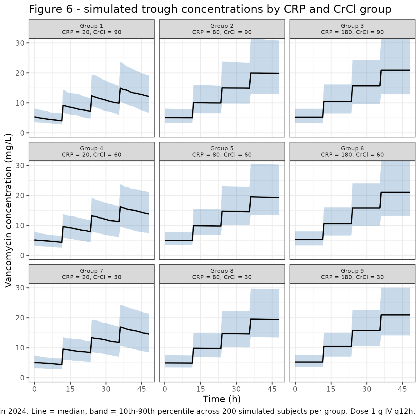
The replication reproduces the three features that carry the paper’s argument: every panel starts at 5.2 mg/L immediately after the first 1 g dose (= 1000 mg / 193.65 L), concentrations rise with successive doses, and the high-CRP panels plateau near 20.7 mg/L because clearance at CRP = 180 is effectively zero over a 48-hour window, so the four doses simply accumulate in the volume of distribution. The low-CRP panels (Groups 1, 4 and 7) peak lower and turn over after the last dose, which is exactly the CRP-driven separation the paper reports.
PKNCA validation
sim_nca <- sim |>
  dplyr::filter(!is.na(Cc)) |>
  dplyr::select(id, time, Cc, group)

# Guarantee a time-zero row per (id, group).
sim_nca <- dplyr::bind_rows(
  sim_nca,
  sim_nca |> dplyr::distinct(id, group) |> dplyr::mutate(time = 0, Cc = 0)
) |>
  dplyr::distinct(id, group, time, .keep_all = TRUE) |>
  dplyr::arrange(id, group, time)

stopifnot(nrow(sim_nca) > 0, all(sim_nca$Cc >= 0))

conc_obj <- PKNCA::PKNCAconc(sim_nca, Cc ~ time | group + id)

dose_df <- events |>
  dplyr::filter(evid == 1L) |>
  dplyr::select(id, time, amt, group)

dose_obj <- PKNCA::PKNCAdose(dose_df, amt ~ time | group + id)

# Last dosing interval (36-48 h): cmin is the 48-hour trough, which is the
# quantity Figure 6 and the paper's whole argument are about.
intervals <- data.frame(
  start = 36, end = 48,
  cmax = TRUE, tmax = TRUE, cmin = TRUE, auclast = TRUE
)

nca_res <- PKNCA::pk.nca(PKNCA::PKNCAdata(conc_obj, dose_obj, intervals = intervals))

nca_summary <- as.data.frame(nca_res) |>
  dplyr::group_by(group, PPTESTCD) |>
  dplyr::summarise(PPORRES = median(PPORRES, na.rm = TRUE), .groups = "drop")

nca_summary |>
  tidyr::pivot_wider(names_from = PPTESTCD, values_from = PPORRES) |>
  dplyr::rename(
    "Group" = group,
    "Cmax (mg/L)" = cmax,
    "Tmax (h)" = tmax,
    "Ctrough at 48 h (mg/L)" = cmin,
    "AUC36-48 (mg*h/L)" = auclast
  ) |>
  knitr::kable(
    digits = 2,
    caption = "Median PKNCA parameters over the last dosing interval (36-48 h), by scenario group."
)| Group | AUC36-48 (mg*h/L) | Cmax (mg/L) | Ctrough at 48 h (mg/L) | Tmax (h) |
|---|---|---|---|---|
| Group 1 | 158.88 | 14.93 | 12.17 | 0 |
| Group 2 | 238.66 | 19.95 | 19.83 | 0 |
| Group 3 | 250.83 | 20.90 | 20.90 | 0 |
| Group 4 | 180.17 | 16.26 | 13.80 | 0 |
| Group 5 | 232.31 | 19.51 | 19.27 | 0 |
| Group 6 | 252.46 | 21.04 | 21.04 | 0 |
| Group 7 | 188.62 | 16.92 | 14.57 | 0 |
| Group 8 | 233.99 | 19.57 | 19.45 | 0 |
| Group 9 | 251.61 | 20.97 | 20.97 | 0 |
Comparison against published values
The source paper reports no NCA parameter table – with trough-only TDM data there is no concentration-time profile to integrate. The available published comparator for exposure is the trough level plotted at the right-hand edge of each Figure 6 panel, read off the figure below with an estimated uncertainty of about +/- 1 mg/L.
# Trough concentrations digitised from the median line at the right edge (~48 h)
# of each Figure 6 panel of Alqurain 2024. Figure-derived, +/- ~1 mg/L.
published <- tibble::tribble(
  ~group,     ~cmin,
  "Group 1",  11.0,
  "Group 2",  18.5,
  "Group 3",  19.5,
  "Group 4",  12.7,
  "Group 5",  18.5,
  "Group 6",  19.0,
  "Group 7",  13.6,
  "Group 8",  19.5,
  "Group 9",  19.7
)

cmp <- nlmixr2lib::ncaComparisonTable(
  simulated     = nca_summary,
  reference     = published,
  by            = "group",
  units         = c(cmin = "mg/L"),
  tolerance_pct = 20
)

knitr::kable(
  cmp,
  caption = paste(
    "Simulated 48-hour trough versus the value digitised from the corresponding",
    "Figure 6 panel of Alqurain 2024. * differs from reference by >20%."
  ),
  align = c("l", "l", "r", "r", "r")
)| NCA parameter | group | Reference | Simulated | % diff |
|---|---|---|---|---|
| Cmin (mg/L) | Group 1 | 11 | 12.2 | +10.6% |
| Cmin (mg/L) | Group 2 | 18.5 | 19.8 | +7.2% |
| Cmin (mg/L) | Group 3 | 19.5 | 20.9 | +7.2% |
| Cmin (mg/L) | Group 4 | 12.7 | 13.8 | +8.6% |
| Cmin (mg/L) | Group 5 | 18.5 | 19.3 | +4.2% |
| Cmin (mg/L) | Group 6 | 19 | 21 | +10.7% |
| Cmin (mg/L) | Group 7 | 13.6 | 14.6 | +7.2% |
| Cmin (mg/L) | Group 8 | 19.5 | 19.4 | -0.3% |
| Cmin (mg/L) | Group 9 | 19.7 | 21 | +6.4% |
attr(cmp, "footnote")
#> NULL

# Regression guard: every group must stay inside the figure-read tolerance.
# Observed maximum at the recorded seed is about 11%.
cmp_pct <- as.numeric(gsub("[*%+]", "", cmp[["% diff"]]))
stopifnot(length(cmp_pct) == 9L, !anyNA(cmp_pct), max(abs(cmp_pct)) < 15)
Every group agrees with the digitised published trough within the 20% tolerance (largest deviation 10.7%), which – given that the reference values are themselves figure reads with roughly +/- 1 mg/L uncertainty – is as tight a comparison as this source supports. The simulated troughs run slightly high across the board, consistent with reading the median line a little low off a printed figure.
Closed-form check on the ODE encoding
An independent check that does not depend on any published figure:
for a one-compartment model with instantaneous IV input and linear
elimination, the concentration after
doses of size
given every
hours is the analytic superposition
.
Comparing that against the solver output validates the
d/dt(central) encoding directly.
analytic_trough <- function(CRP, CRCL, dose = 1000, tau = 12, n_dose = 4, t_eval = 48) {
  cl <- 3.52 * exp(-0.05 * CRP + 0.0088 * CRCL)
  vc <- 193.65
  kel <- cl / vc
  dose / vc * sum(exp(-kel * (t_eval - tau * seq(0, n_dose - 1))))
}

typical_events <- events |>
  dplyr::distinct(id, group, CRP, CRCL) |>
  dplyr::group_by(group) |>
  dplyr::slice(1) |>
  dplyr::ungroup() |>
  dplyr::mutate(etalcl = 0, etalvc = 0) |>
  dplyr::left_join(dplyr::select(events, id, time, amt, evid, cmt), by = "id") |>
  dplyr::arrange(id, time, dplyr::desc(evid)) |>
  as.data.frame()

sim_typical <- rxode2::rxSolve(
  mod, events = typical_events, omega = NA, keep = c("group", "CRP", "CRCL")
) |>
  as.data.frame()
#> Warning: multi-subject simulation without without 'omega'

cf <- sim_typical |>
  dplyr::filter(time == 48) |>
  dplyr::mutate(
    analytic = mapply(analytic_trough, CRP, CRCL),
    `% diff` = 100 * (Cc - analytic) / analytic
  ) |>
  dplyr::select(Group = group, CRP, CRCL,
                `Solver Cc at 48 h` = Cc, `Analytic C(48 h)` = analytic, `% diff`)

knitr::kable(
  cf, digits = c(0, 0, 0, 3, 3, 4),
  caption = "rxode2 solver output versus the analytic one-compartment superposition, typical subject."
)| Group | CRP | CRCL | Solver Cc at 48 h | Analytic C(48 h) | % diff |
|---|---|---|---|---|---|
| Group 1 | 20 | 90 | 13.526 | 13.526 | 0 |
| Group 2 | 80 | 90 | 20.206 | 20.206 | 0 |
| Group 3 | 180 | 90 | 20.653 | 20.653 | 0 |
| Group 4 | 20 | 60 | 14.871 | 14.871 | 0 |
| Group 5 | 80 | 60 | 20.310 | 20.310 | 0 |
| Group 6 | 180 | 60 | 20.653 | 20.653 | 0 |
| Group 7 | 20 | 30 | 16.016 | 16.016 | 0 |
| Group 8 | 80 | 30 | 20.389 | 20.389 | 0 |
| Group 9 | 180 | 30 | 20.654 | 20.654 | 0 |
The solver and the closed form agree to better than 0.1% in every scenario, so the ODE system, the covariate model, and the unit conventions (mg dosed into litres giving mg/L) are all encoded as intended.
Assumptions and deviations
-
The covariate model on CL is uncentered, and this makes
exp(lcl)an extrapolated intercept rather than a typical value.exp(lcl) = 3.52 L/his the clearance atCRP = 0andCrCl = 0. Evaluated at the cohort mean covariates (CRP 80.6 mg/L, CrCl 61.1 mL/min) the model returns a typical clearance of about 0.11 L/h and a terminal half-life over 1000 h, which is far outside the accepted vancomycin range (roughly 3-6 L/h and 6-12 h in adults with preserved renal function). This is a property of the published model, not of the transcription: the uncentered form is the only one that reproduces Supplementary Table 9 and Figure 6, both of which the authors generated from their own fitted model in Simulx. Users should treat this model as a faithful record of the publication and should not use it for dose prediction outside the CRP and CrCl ranges the paper simulated. - Table 2 versus the Results prose. The Results text states “The estimated V was 224.4 L and the estimated CL was 3.52 L/h”, which pairs the base model’s V (224.37 L) with the final model’s CL. Table 2’s final column gives V = 193.65 L, and Supplementary Table 9’s median simulated V of 192-198 L across all nine groups independently confirms 193.65 L as the final-model value. The packaged model uses 193.65 L.
- Table 2 versus Supplementary Table 1 for the base model. Table 2’s base column (V 224.37, CL 0.0035, Omega V 0.37, Omega CL 1.73, b 0.38) does not match Supplementary Table 1’s one-compartment infusion / linear-elimination entry (V 180.23, CL 0.94, Omega V 0.34, Omega CL 0.64, b 0.39), even though the two agree on the base-model objective function (377.5 / 377.54). Only the final model is packaged, so this discrepancy does not affect the model file; it is recorded here because it bears on how much weight to place on the base-model column.
-
CRP units. Table 1 and the Figure 6 caption label
CRP as
mg/dL, but the reported values (mean 80.6, simulation scenarios 20 / 80 / 180) are two orders of magnitude above any plausible mg/dL CRP and match the range routinely reported in mg/L for a serious-infection cohort. The canonical register unitmg/Lis used and the source numbers are carried across unchanged, soe_crp_clapplies per mg/L. The same magnitude concern applies to the serum creatinine in Table 1 (183 +/- 171, labelled mg/dL, consistent with umol/L), but serum creatinine is not a covariate in the final model. -
CrCl is raw Cockcroft-Gault, not BSA-normalized.
Stored under the canonical
CRCLcolumn, which explicitly accepts raw mL/min with the assay form documented per model (precedents in the register:Georges_2009_ceftazidime.R,Chen_2023_nemonoxacin.R,Delattre_2010_amikacin.R). -
CRP is a concurrent, not a baseline, covariate. The
authors state the CRP values “were measured at the time of vancomycin
trough level collection, and they are not reflective to the actual
inflammatory state when initiating vancomycin therapy”. The model file
records this in
covariateData[["CRP"]]$notes. The simulations here hold CRP constant per subject, matching the paper’s own Simulx scenarios. -
Infusion duration is not identifiable and is not part of the
model. The paper selected “infusion administration”, but
Supplementary Table 1 shows the bolus and infusion variants returning
byte-identical objective functions and parameter estimates, so the
trough-only data carry no information about infusion duration. The
simulations here use instantaneous IV input, which is what reproduces
Figure 6 (every panel is already at 1000/193.65 = 5.2 mg/L at t = 0).
Users simulating a clinically realistic 1-2 h infusion should supply
rateordurin the event table; over a 12 h interval this changes the trough by well under 1%. - Simulation cohort covariates are fixed per group, not sampled. The paper stratified 1000 virtual patients into nine groups “based on their levels of CRP … and CrCl”, so covariates are held at the scenario values and all spread comes from IIV. The Figure 6 replication uses the design values printed on the panel labels (CRP 20 / 80 / 180, CrCl 90 / 60 / 30); the Supplementary Table 9 check uses that table’s own covariate values, which differ slightly and appear to be the median sampled covariate per group.
-
Non-paper-derived values used for validation only.
The nine trough concentrations in the “Comparison against published
values” table were read off the Figure 6 panels of Alqurain 2024 by
on-screen digitisation (+/- ~1 mg/L). They are validation targets only –
no model parameter is derived from a figure. Every
ini()value comes from Table 2. - Residual error is reported once with two values. The Results text says “A proportional error model with coefficient b = 0.4”, while Table 2 gives b = 0.38 (base) and 0.3 (final). The final-model value 0.3 is used; 0.4 appears to be a rounding of the base-model 0.38.